9_Transcriptome Assembly – BCH709 Introduction to Bioinformatics

Conda env

conda activate rnaseq

File prepare

mkdir -p /data/gpfs/assoc/bch709-1/<YOURID>/rnaseq_slurm/fastq

cd /data/gpfs/assoc/bch709-1/<YOURID>/rnaseq_slurm/fastq

cp /data/gpfs/assoc/bch709-1/Course_material/2020/RNASeq_raw_fastq/*.gz .

cd ../
ls

pronghorn

 nano submit.sh

#!/bin/bash
#SBATCH --job-name=test
#SBATCH --cpus-per-task=16
#SBATCH --time=10:00
#SBATCH --account=cpu-s2-bch709-1 
#SBATCH --partition=cpu-s2-core-0
#SBATCH --mem-per-cpu=1g
#SBATCH --mail-type=begin
#SBATCH --mail-type=end
#SBATCH --mail-type=fail
#SBATCH --mail-user=<YOUR ID>@unr.edu
echo "Hello Pronghorn"
seq 1 8000

would request one CPU for 10 minutes, along with 1g of RAM, in the default queue. When started, the job would run a first job step srun hostname, which will launch the UNIX command hostname on the node on which the requested CPU was allocated. Then, a second job step will start the sleep command. Note that the –job-name parameter allows giving a meaningful name to the job and the –output parameter defines the file to which the output of the job must be sent.

Once the submission script is written properly, you need to submit it to slurm through the sbatch command, which, upon success, responds with the jobid attributed to the job. (The dollar sign below is the shell prompt)

$ chmod 775 submit.sh
$ sbatch submit.sh
sbatch: Submitted batch job

Slurm Quick Start Tutorial

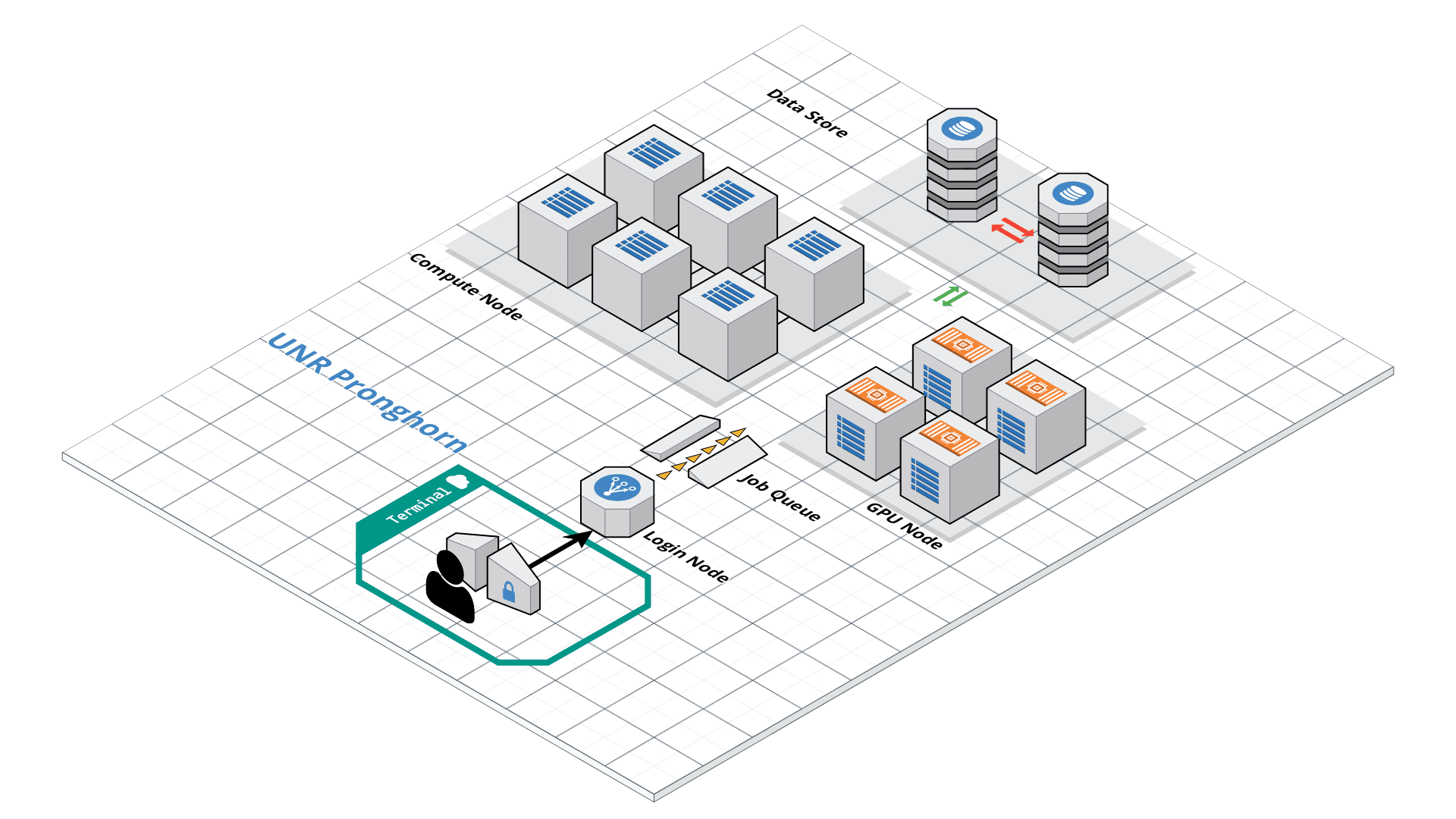
Resource sharing on a supercomputer dedicated to technical and/or scientific computing is often organized by a piece of software called a resource manager or job scheduler. Users submit jobs, which are scheduled and allocated resources (CPU time, memory, etc.) by the resource manager.

Slurm is a resource manager and job scheduler designed to do just that, and much more. It was originally created by people at the Livermore Computing Center, and has grown into a full-fledge open-source software backed up by a large community, commercially supported by the original developers, and installed in many of the Top500 supercomputers.

Gathering information Slurm offers many commands you can use to interact with the system. For instance, the sinfo command gives an overview of the resources offered by the cluster, while the squeue command shows to which jobs those resources are currently allocated.

By default, sinfo lists the partitions that are available. A partition is a set of compute nodes (computers dedicated to… computing) grouped logically. Typical examples include partitions dedicated to batch processing, debugging, post processing, or visualization.

sinfo

Show the State of Nodes

sinfo --all

PARTITION      AVAIL  TIMELIMIT  NODES  STATE NODELIST
cpu-s2-core-0     up 14-00:00:0      2    mix cpu-[8-9]
cpu-s2-core-0     up 14-00:00:0      7  alloc cpu-[1-2,4-6,78-79]
cpu-s2-core-0     up 14-00:00:0     44   idle cpu-[0,3,7,10-47,64,76-77]
cpu-s3-core-0*    up    2:00:00      2    mix cpu-[8-9]
cpu-s3-core-0*    up    2:00:00      7  alloc cpu-[1-2,4-6,78-79]
cpu-s3-core-0*    up    2:00:00     44   idle cpu-[0,3,7,10-47,64,76-77]
gpu-s2-core-0     up 14-00:00:0     11   idle gpu-[0-10]
cpu-s6-test-0     up      15:00      2   idle cpu-[65-66]
cpu-s1-pgl-0      up 14-00:00:0      1    mix cpu-49
cpu-s1-pgl-0      up 14-00:00:0      1  alloc cpu-48
cpu-s1-pgl-0      up 14-00:00:0      2   idle cpu-[50-51]

In the above example, we see two partitions, named batch and debug. The latter is the default partition as it is marked with an asterisk. All nodes of the debug partition are idle, while two of the batch partition are being used.

The sinfo command also lists the time limit (column TIMELIMIT) to which jobs are subject. On every cluster, jobs are limited to a maximum run time, to allow job rotation and let every user a chance to see their job being started. Generally, the larger the cluster, the smaller the maximum allowed time. You can find the details on the cluster page.

You can actually specify precisely what information you would like sinfo to output by using its –format argument. For more details, have a look at the command manpage with man sinfo.

sinfo advance

sinfo $OPTIONS -o "%13n %8t %4c %8z %15C %8O %8m %8G %18P %f"  | egrep s2

squeue

The squeue command shows the list of jobs which are currently running (they are in the RUNNING state, noted as ‘R’) or waiting for resources (noted as ‘PD’, short for PENDING).

squeue

             JOBID PARTITION     NAME     USER ST       TIME  NODES NODELIST(REASON)
            983204 cpu-s2-co    neb_K jzhang23  R 6-09:05:47      1 cpu-6
            983660 cpu-s2-co   RT3.sl yinghanc  R   12:56:17      1 cpu-9
            983659 cpu-s2-co   RT4.sl yinghanc  R   12:56:21      1 cpu-8
            983068 cpu-s2-co Gd-bound   dcantu  R 7-06:16:01      2 cpu-[78-79]
            983067 cpu-s2-co Gd-unbou   dcantu  R 1-17:41:56      2 cpu-[1-2]
            983472 cpu-s2-co   ub-all   dcantu  R 3-10:05:01      2 cpu-[4-5]
            982604 cpu-s1-pg     wrap     wyim  R 12-14:35:23      1 cpu-49
            983585 cpu-s1-pg     wrap     wyim  R 1-06:28:29      1 cpu-48
            983628 cpu-s1-pg     wrap     wyim  R   13:44:46      1 cpu-49

SBATCH

Now the question is: How do you create a job?

A job consists in two parts: resource requests and job steps. Resource requests consist in a number of CPUs, computing expected duration, amounts of RAM or disk space, etc. Job steps describe tasks that must be done, software which must be run.

The typical way of creating a job is to write a submission script. A submission script is a shell script, e.g. a Bash script, whose comments, if they are prefixed with SBATCH, are understood by Slurm as parameters describing resource requests and other submissions options. You can get the complete list of parameters from the sbatch manpage man sbatch.

Important

The SBATCH directives must appear at the top of the submission file, before any other line except for the very first line which should be the shebang (e.g. #!/bin/bash). The script itself is a job step. Other job steps are created with the srun command. For instance, the following script, hypothetically named submit.sh,

Submit job

chmod 775 trim.sh
sbatch trim.sh

Trimming job running

Trimming Practice
- Make rnaseq_slurm/fastq folder under /data/gpfs/assoc/bch709-1/YOURID/
- Change directory to the folder rnaseq_slurm/fastq
- Copy all fastq.gz files in /data/gpfs/assoc/bch709-1/Course_material/2020/RNASeq_raw_fastq to rnaseq_slurm/fastq folder

Sample	Replication	Forward (read1)	Reverse (read2)
Wildtype	Rep1	WT1_R1.fastq.gz	WT1_R2.fastq.gz
Wildtype	Rep2	WT2_R1.fastq.gz	WT2_R2.fastq.gz
Wildtype	Rep3	WT3_R1.fastq.gz	WT3_R2.fastq.gz
Stressed (drought)	Rep1	DT1_R1.fastq.gz	DT1_R2.fastq.gz
Stressed (drought)	Rep2	DT2_R1.fastq.gz	DT2_R2.fastq.gz
Stressed (drought)	Rep3	DT3_R1.fastq.gz	DT3_R2.fastq.gz

Run Trim-Galore and process MultiQC
Generate 6 trimmed output from MultiQC and upload html file to WebCanvas.

Run trimming

pwd
nano trim.sh

#!/bin/bash
#SBATCH --job-name=<TRIM>
#SBATCH --time=15:00
#SBATCH --account=cpu-s2-bch709-1 
#SBATCH --partition=cpu-s2-core-0
#SBATCH --cpus-per-task=8
#SBATCH --mem-per-cpu=4g
#SBATCH --mail-type=fail
#SBATCH --mail-type=begin
#SBATCH --mail-type=end
#SBATCH --mail-user=<YOUR ID>@unr.edu
#SBATCH --output=<TRIM>.out


trim_galore --paired   --three_prime_clip_R1 20 --three_prime_clip_R2 20 --cores 8  --max_n 40  --gzip -o trim /data/gpfs/assoc/bch709-1/<YOURID>/rnaseq_slurm/fastq/DT1_R1.fastq.gz  /data/gpfs/assoc/bch709-1/<YOURID>/rnaseq_slurm/fastq/DT1_R2.fastq.gz

trim_galore --paired   --three_prime_clip_R1 20 --three_prime_clip_R2 20 --cores 16  --max_n 40  --gzip -o trim /data/gpfs/assoc/bch709-1/<YOURID>/rnaseq_slurm/fastq/DT2_R1.fastq.gz  /data/gpfs/assoc/bch709-1/<YOURID>/rnaseq_slurm/fastq/DT2_R2.fastq.gz
.
.
.
.
.
.

squeue

The squeue command shows the list of jobs which are currently running (they are in the RUNNING state, noted as ‘R’) or waiting for resources (noted as ‘PD’, short for PENDING).

squeue

             JOBID PARTITION     NAME     USER ST       TIME  NODES NODELIST(REASON)
            983204 cpu-s2-co    neb_K jzhang23  R 6-09:05:47      1 cpu-6
            983660 cpu-s2-co   RT3.sl yinghanc  R   12:56:17      1 cpu-9
            983659 cpu-s2-co   RT4.sl yinghanc  R   12:56:21      1 cpu-8
            983068 cpu-s2-co Gd-bound   dcantu  R 7-06:16:01      2 cpu-[78-79]
            983067 cpu-s2-co Gd-unbou   dcantu  R 1-17:41:56      2 cpu-[1-2]
            983472 cpu-s2-co   ub-all   dcantu  R 3-10:05:01      2 cpu-[4-5]
            982604 cpu-s1-pg     wrap     wyim  R 12-14:35:23      1 cpu-49
            983585 cpu-s1-pg     wrap     wyim  R 1-06:28:29      1 cpu-48
            983628 cpu-s1-pg     wrap     wyim  R   13:44:46      1 cpu-49

Loop submission

import os

def mkdir_p(dir):
    '''make a directory (dir) if it doesn't exist'''
    if not os.path.exists(dir):
        os.mkdir(dir)


job_directory = "%s/.job" %os.getcwd()
scratch = scratch = os.getcwd()
data_dir = os.path.join(scratch, 'trim')

# Make top level directories
mkdir_p(data_dir)
mkdir_p(job_directory)
samples=["DT1","DT2", "DT3", "WT1", "WT2","WT3"]

for fastq in samples:

    job_file = os.path.join(job_directory,"%s.job" % fastq)
    fastq_data = os.path.join(data_dir, fastq)

    # Create fastq directories
    mkdir_p(fastq_data)

    with open(job_file, 'w') as fh:
        fh.writelines("#!/bin/bash\n")
        fh.writelines("#SBATCH --job-name=%s.job\n" % fastq)
        fh.writelines("#SBATCH --output=%s.out\n" % fastq)
        fh.writelines("#SBATCH --error=%s.err\n" % fastq)
        fh.writelines("#SBATCH --time=15:00\n")
        fh.writelines("#SBATCH --account=cpu-s2-bch709-1\n")
        fh.writelines("#SBATCH --partition=cpu-s2-core-0\n")
        fh.writelines("#SBATCH --cpus-per-task=16\n")
        fh.writelines("#SBATCH --mem-per-cpu=4g\n")
        fh.writelines("#SBATCH --mail-type=fail\n")
        fh.writelines("#SBATCH --mail-type=begin\n")
        fh.writelines("#SBATCH --mail-type=end\n")
        fh.writelines("#SBATCH --cpus-per-task=16\n")
        fh.writelines("#SBATCH --mail-type=ALL\n")
        fh.writelines("#SBATCH --mail-user=wyim@unr.edu\n")
        fh.writelines("trim_galore --paired   --three_prime_clip_R1 20 --three_prime_clip_R2 20 --cores 16  --max_n 40  --gzip -o trim /data/gpfs/assoc/bch709-1/wyim/rnaseq_slurm/fastq/%s_R1.fastq.gz  /data/gpfs/assoc/bch709-1/wyim/rnaseq_slurm/fastq/%s_R2.fastq.gz\n" % (fastq,fastq))

    os.system("sbatch %s" %job_file)

#!/bin/bash

# We assume running this from the script directory
job_directory=$PWD/.job
data_dir="${SCRATCH}/trim"

fastq=("DT1" "DT2" "DT3" "WT1" "WT2" "WT3")

for fastq in ${fastq[@]}; do

    job_file="${job_directory}/${fastq}.job"

    echo "#!/bin/bash
#SBATCH --job-name=${fastq}.job
#SBATCH --output=${fastq}.out
#SBATCH --error=${fastq}.err
#SBATCH --time=15:00
#SBATCH --account=cpu-s2-bch709-1 
#SBATCH --partition=cpu-s2-core-0
#SBATCH --cpus-per-task=16
#SBATCH --mem-per-cpu=4g
#SBATCH --mail-type=fail
#SBATCH --mail-type=begin
#SBATCH --mail-type=end
#SBATCH --cpus-per-task=16
#SBATCH --mail-type=ALL
#SBATCH --mail-user=wyim@unr.edu
trim_galore --paired --three_prime_clip_R1 20 --three_prime_clip_R2 20 --cores 16  --max_n 40  --gzip -o trim /data/gpfs/assoc/bch709-1/wyim/rnaseq_slurm/fastq/${fastq}_R1.fastq.gz  /data/gpfs/assoc/bch709-1/wyim/rnaseq_slurm/fastq/${fastq}_R2.fastq.gz"> $job_file

sbatch $job_file

done

Youtube Video for Slurm

https://www.youtube.com/watch?v=U42qlYkzP9k

https://www.youtube.com/watch?v=LRJMQO7Ercw

More Slurm command

# Show the overall status of each partition
sinfo

# Submit a job
sbatch <JOBFILE>

# See the entire job queue
squeue

# See only jobs for a given user
squeue -u <username>

# Count number of running / in queue jobs
squeue -u <username> | wc -l

# Get estimated start times for your jobs (when Sherlock is busy)
squeue --start -u <username>

# Show the status of a currently running job
sstat -j <jobID>

# Show the final status of a finished job
sacct -j <jobID>

# Kill a job with ID $PID
scancel <jobID>

# Kill ALL jobs for a user
scancel -u <username>

PLEASE CHECK YOUR MULTIQC after job running

MultiQC

multiqc  --filename trim  .

Running Trinity

Trinity is run via the script: ‘Trinity’ found in the base installation directory.

Usage info is as follows:

 ###############################################################################
 #
 #     ______  ____   ____  ____   ____  ______  __ __
 #    |      ||    \ |    ||    \ |    ||      ||  |  |
 #    |      ||  D  ) |  | |  _  | |  | |      ||  |  |
 #    |_|  |_||    /  |  | |  |  | |  | |_|  |_||  ~  |
 #      |  |  |    \  |  | |  |  | |  |   |  |  |___, |
 #      |  |  |  .  \ |  | |  |  | |  |   |  |  |     |
 #      |__|  |__|\_||____||__|__||____|  |__|  |____/
 #
 ###############################################################################
 #
 # Required:
 #
 #  --seqType <string>      :type of reads: ( fa, or fq )
 #
 #  --max_memory <string>      :suggested max memory to use by Trinity where limiting can be enabled. (jellyfish, sorting, etc)
 #                            provided in Gb of RAM, ie.  '--max_memory 10G'
 #
 #  If paired reads:
 #      --left  <string>    :left reads, one or more file names (separated by commas, not spaces)
 #      --right <string>    :right reads, one or more file names (separated by commas, not spaces)
 #
 #  Or, if unpaired reads:
 #      --single <string>   :single reads, one or more file names, comma-delimited (note, if single file contains pairs, can use flag: --run_as_paired )
 #
 #  Or,
 #      --samples_file <string>         tab-delimited text file indicating biological replicate relationships.
 #                                   ex.
 #                                        cond_A    cond_A_rep1    A_rep1_left.fq    A_rep1_right.fq
 #                                        cond_A    cond_A_rep2    A_rep2_left.fq    A_rep2_right.fq
 #                                        cond_B    cond_B_rep1    B_rep1_left.fq    B_rep1_right.fq
 #                                        cond_B    cond_B_rep2    B_rep2_left.fq    B_rep2_right.fq
 #
 #                      # if single-end instead of paired-end, then leave the 4th column above empty.
 #
 ####################################
 ##  Misc:  #########################
 #
 #  --SS_lib_type <string>          :Strand-specific RNA-Seq read orientation.
 #                                   if paired: RF or FR,
 #                                   if single: F or R.   (dUTP method = RF)
 #                                   See web documentation.
 #
 #  --CPU <int>                     :number of CPUs to use, default: 2
 #  --min_contig_length <int>       :minimum assembled contig length to report
 #                                   (def=200)
 #
 #  --long_reads <string>           :fasta file containing error-corrected or circular consensus (CCS) pac bio reads
 #
 #  --genome_guided_bam <string>    :genome guided mode, provide path to coordinate-sorted bam file.
 #                                   (see genome-guided param section under --show_full_usage_info)
 #
 #  --jaccard_clip                  :option, set if you have paired reads and
 #                                   you expect high gene density with UTR
 #                                   overlap (use FASTQ input file format
 #                                   for reads).
 #                                   (note: jaccard_clip is an expensive
 #                                   operation, so avoid using it unless
 #                                   necessary due to finding excessive fusion
 #                                   transcripts w/o it.)
 #
 #  --trimmomatic                   :run Trimmomatic to quality trim reads
 #                                        see '--quality_trimming_params' under full usage info for tailored settings.
 #
 #
 #  --no_normalize_reads            :Do *not* run in silico normalization of reads. Defaults to max. read coverage of 50.
 #                                       see '--normalize_max_read_cov' under full usage info for tailored settings.
 #                                       (note, as of Sept 21, 2016, normalization is on by default)
 #
 #
 #
 #  --output <string>               :name of directory for output (will be
 #                                   created if it doesn't already exist)
 #                                   default( your current working directory: "/Users/bhaas/GITHUB/trinityrnaseq/trinity_out_dir"
 #                                    note: must include 'trinity' in the name as a safety precaution! )
 #
 #  --full_cleanup                  :only retain the Trinity fasta file, rename as ${output_dir}.Trinity.fasta
 #
 #  --cite                          :show the Trinity literature citation
 #
 #  --version                       :reports Trinity version (BLEEDING_EDGE) and exits.
 #
 #  --show_full_usage_info          :show the many many more options available for running Trinity (expert usage).
 #
 #
 ###############################################################################
 #
 #  *Note, a typical Trinity command might be:
 #
 #        Trinity --seqType fq --max_memory 50G --left reads_1.fq  --right reads_2.fq --CPU 6
 #
 #
 #    and for Genome-guided Trinity:
 #
 #        Trinity --genome_guided_bam rnaseq_alignments.csorted.bam --max_memory 50G
 #                --genome_guided_max_intron 10000 --CPU 6
 #
 #     see: /Users/bhaas/GITHUB/trinityrnaseq/sample_data/test_Trinity_Assembly/
 #          for sample data and 'runMe.sh' for example Trinity execution
 #
 #     For more details, visit: http://trinityrnaseq.github.io
 #
 ###############################################################################

Trinity performs best with strand-specific data, in which case sense and antisense transcripts can be resolved. For protocols on strand-specific RNA-Seq, see: Borodina T, Adjaye J, Sultan M. A strand-specific library preparation protocol for RNA sequencing. Methods Enzymol. 2011;500:79-98. PubMed PMID: 21943893.

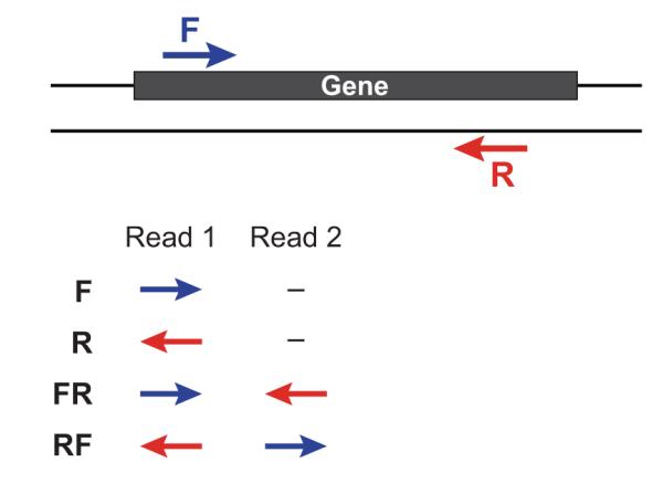
If you have strand-specific data, specify the library type. There are four library types:

Paired reads:
- RF: first read (/1) of fragment pair is sequenced as anti-sense (reverse(R)), and second read (/2) is in the sense strand (forward(F)); typical of the dUTP/UDG sequencing method.
- FR: first read (/1) of fragment pair is sequenced as sense (forward), and second read (/2) is in the antisense strand (reverse)
Unpaired (single) reads:
- F: the single read is in the sense (forward) orientation
- R: the single read is in the antisense (reverse) orientation

By setting the –SS_lib_type parameter to one of the above, you are indicating that the reads are strand-specific. By default, reads are treated as not strand-specific.

strand specific specification

Other important considerations:

Whether you use Fastq or Fasta formatted input files, be sure to keep the reads oriented as they are reported by Illumina, if the data are strand-specific. This is because, Trinity will properly orient the sequences according to the specified library type. If the data are not strand-specific, no worries because the reads will be parsed in both orientations.
If you have both paired and unpaired data, and the data are NOT strand-specific, you can combine the unpaired data with the left reads of the paired fragments. Be sure that the unpaired reads have a /1 as a suffix to the accession value similarly to the left fragment reads. The right fragment reads should all have /2 as the accession suffix. Then, run Trinity using the –left and –right parameters as if all the data were paired.
If you have multiple paired-end library fragment sizes, set the ‘–group_pairs_distance’ according to the larger insert library. Pairings that exceed that distance will be treated as if they were unpaired by the Butterfly process.
by setting the ‘–CPU option’, you are indicating the maximum number of threads to be used by processes within Trinity. Note that Inchworm alone will be internally capped at 6 threads, since performance will not improve for this step beyond that setting)

Typical Trinity Command Line

A typical Trinity command for assembling non-strand-specific RNA-seq data would be like so, running the entire process on a single high-memory server (aim for ~1G RAM per ~1M ~76 base Illumina paired reads, but often much less memory is required):

Run Trinity like so:

 Trinity --seqType fq --max_memory 50G \
         --left reads_1.fq.gz  --right reads_2.fq.gz --CPU 6

If you have multiple sets of fastq files, such as corresponding to multiple tissue types or conditions, etc., you can indicate them to Trinity like so:

 Trinity --seqType fq --max_memory 50G  \
         --left condA_1.fq.gz,condB_1.fq.gz,condC_1.fq.gz \
         --right condA_2.fq.gz,condB_2.fq.gz,condC_2.fq.gz \
         --CPU 6

or better yet, create a ‘samples.txt’ file that describes the data like so:

 #      --samples_file <string>         tab-delimited text file indicating biological replicate relationships.
 #                                   ex.
 #                                        cond_A    cond_A_rep1    A_rep1_left.fq    A_rep1_right.fq
 #                                        cond_A    cond_A_rep2    A_rep2_left.fq    A_rep2_right.fq
 #                                        cond_B    cond_B_rep1    B_rep1_left.fq    B_rep1_right.fq
 #                                        cond_B    cond_B_rep2    B_rep2_left.fq    B_rep2_right.fq

This same samples file can then be used later on with other downstream analysis steps, including expression quantification and differential expression analysis.

note that fastq files can be gzip-compressed as shown above, in which case they should require a ‘.gz’ extension.

Trinity run


nano trinity.sh

###^ means CTRL key ###M- means ALT key

#!/bin/bash
#SBATCH --job-name=<TRINITY>
#SBATCH --time=15:00
#SBATCH --account=cpu-s2-bch709-0
#SBATCH --partition=cpu-s2-core-0
#SBATCH --cpus-per-task=8
#SBATCH --mem=80g
#SBATCH --mail-type=fail
#SBATCH --mail-type=begin
#SBATCH --mail-type=end
#SBATCH --mail-user=<YOUR ID>@unr.edu
#SBATCH --output=<TRINITY>.out


Trinity --seqType fq  --CPU 24 --max_memory 80G --left trim/DT1_R1_val_1.fq.gz,trim/DT2_R1_val_1.fq.gz,trim/DT3_R1_val_1.fq.gz,trim/WT1_R1_val_1.fq.gz,trim/WT2_R1_val_1.fq.gz,trim/WT3_R1_val_1.fq.gz --right trim/DT1_R2_val_2.fq.gz,trim/DT2_R2_val_2.fq.gz,trim/DT3_R2_val_2.fq.gz,trim/WT1_R2_val_2.fq.gz,trim/WT2_R2_val_2.fq.gz,trim/WT3_R2_val_2.fq.gz

Please consider relative path and absolute path

Submit job

chmod 775 trinity.sh

sbatch trinity.sh

de Bruijn

de Bruijn graph construction

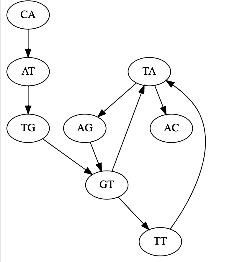
Draw (by hand) the de Bruijn graph for the following reads using k=3 (assume all reads are from the forward strand, no sequencing errors) AGT
ATG
CAT
GTA
GTT
TAC
TAG
TGT TTA

[('AG', 'GT'),
 ('AT', 'TG'),
 ('CA', 'AT'),
 ('GT', 'TA'),
 ('GT', 'TT'),
 ('TA', 'AC'),
 ('TA', 'AG'),
 ('TG', 'GT'),
 ('TT', 'TA')]

debj_graph

python code

https://colab.research.google.com/drive/12AIJ21eGQ2npxeHcU3h4fT7OxEzxxzin#scrollTo=FN4AvrS0g3uN

Please check the result

cd /data/gpfs/assoc/bch709-1/<YOURID>/rnaseq_slurm/trinity_out_dir/

egrep -c ">" /data/gpfs/assoc/bch709-1/<YOURID>/rnaseq_slurm/trinity_out_dir/Trinity.fasta 

TrinityStats.pl /data/gpfs/assoc/bch709-1/<YOURID>/rnaseq_slurm/trinity_out_dir/Trinity.fasta  >> <YOURID>.trinity.stat

<YOURID>.trinity.stat

RNA-Seq reads Count Analysis

pwd
### Your current location is 
## /data/gpfs/assoc/bch709-1/wyim/rnaseq_slurm
align_and_estimate_abundance.pl


nano reads_count.sh

RNA-Seq reads Count Analysis job script

#!/bin/bash
#SBATCH --job-name=<JOBNAME>
#SBATCH --cpus-per-task=16
#SBATCH --time=15:00
#SBATCH --mem=16g
#SBATCH --mail-type=begin
#SBATCH --mail-type=end
#SBATCH --mail-type=fail
#SBATCH --mail-user=<YOUR ID>@unr.edu
#SBATCH -o <JOBNAME>.out # STDOUT
#SBATCH -e <JOBNAME>.err # STDERR
#SBATCH --account=cpu-s2-bch709-1 
#SBATCH --partition=cpu-s2-core-0


align_and_estimate_abundance.pl --transcripts trinity_out_dir/Trinity.fasta --seqType fq --left trim/DT1_R1_val_1.fq.gz --right trim/DT1_R2_val_2.fq.gz --est_method RSEM --aln_method bowtie2 --trinity_mode --prep_reference --output_dir rsem_outdir_test  --thread_count  16

RSEM

Job submission

sbatch reads_count.sh

Job check

squeue

Job running check

## do ```ls``` first
ls
cat slurm_<JOBID>.out 

RSEM results check

less rsem_outdir_test/RSEM.genes.results

Expression values and Normalization

CPM, RPKM, FPKM, TPM, RLE, MRN, Q, UQ, TMM, VST, RLOG, VOOM … Too many…

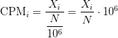
CPM: Controls for sequencing depth when dividing by total count. Not for within-sample comparison or DE.

Counts per million (CPM) mapped reads are counts scaled by the number of fragments you sequenced (N) times one million. This unit is related to the FPKM without length normalization and a factor of 10^3:
CPM

RPKM/FPKM: Controls for sequencing depth and gene length. Good for technical replicates, not good for sample-sample due to compositional bias. Assumes total RNA output is same in all samples. Not for DE.

TPM: Similar to RPKM/FPKM. Corrects for sequencing depth and gene length. Also comparable between samples but no correction for compositional bias.

TMM/RLE/MRN: Improved assumption: The output between samples for a core set only of genes is similar. Corrects for compositional bias. Used for DE. RLE and MRN are very similar and correlates well with sequencing depth. edgeR::calcNormFactors() implements TMM, TMMwzp, RLE & UQ. DESeq2::estimateSizeFactors implements median ratio method (RLE). Does not correct for gene length.

VST/RLOG/VOOM: Variance is stabilised across the range of mean values. For use in exploratory analyses. Not for DE. vst() and rlog() functions from DESeq2. voom() function from Limma converts data to normal distribution.

geTMM: Gene length corrected TMM.

For DEG using DEG R packages (DESeq2, edgeR, Limma etc), use raw counts
For visualisation (PCA, clustering, heatmaps etc), use TPM or TMM
For own analysis with gene length correction, use TPM (maybe geTMM?)
Other solutions: spike-ins/house-keeping genes

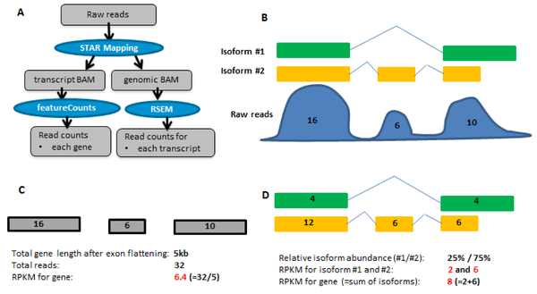
FPKM

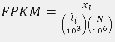
X = mapped reads count N = number of reads L = Length of transcripts

head -n 2 rsem_outdir_test/RSEM.genes.results

‘length’ is this transcript’s sequence length (poly(A) tail is not counted). ‘effective_length’ counts only the positions that can generate a valid fragment.

Reads count

samtools flagstat rsem_outdir_test/bowtie2.bam

cat rsem_outdir_test/RSEM.genes.results | egrep -v FPKM | awk '{ sum+=$5} END {print sum}'

Call Python

python

FPKM

Fragments per Kilobase of transcript per million mapped reads

X = 2012.00
Number_Reads_mapped = 559779
Length = 650.92
fpkm= X*(1000/Length)*(1000000/Number_Reads_mapped)
fpkm

ten to the ninth power = 10**9

fpkm=X/(Number_Reads_mapped*Length)*10**9
fpkm

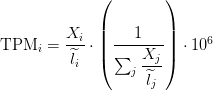
TPM

Transcripts Per Million

TPM

TPM2

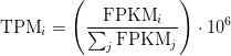
Sum of FPKM

cat rsem_outdir_test/RSEM.genes.results | egrep -v FPKM | awk '{ sum+=$7} END {print sum}'

TPM calculation from FPKM

FPKM = 5521.839239919676
SUM_FPKM = 931616
TPM=(FPKM/SUM_FPKM)*10**6
TPM

TPM calculation from reads count

cat rsem_outdir_test/RSEM.genes.results | egrep -v FPKM | awk '{ sum+=$5/$4} END {print sum}'

sum_count_per_length = 521.494
X = 2012.00
Length = 650.92
TPM = (X/Length)*(1/sum_count_per_length )*10**6
TPM

Paper read

Li et al., 2010, RSEM

Dillies et al., 2013

DEG calculation

Conda env

conda activate rnaseq

File prepare


cd /data/gpfs/assoc/bch709-1/<YOURID>/rnaseq_slurm/

Type sample file

nano sample.txt

###^ means CTRL key ###M- means ALT key

WT<TAB>WT_REP1<TAB>trim/WT1_R1_val_1.fq.gz<TAB>trim/WT1_R2_val_2.fq.gz
WT<TAB>WT_REP2<TAB>trim/WT2_R1_val_1.fq.gz<TAB>trim/WT2_R2_val_2.fq.gz
WT<TAB>WT_REP3<TAB>trim/WT3_R1_val_1.fq.gz<TAB>trim/WT3_R2_val_2.fq.gz
DT<TAB>DT_REP1<TAB>trim/DT1_R1_val_1.fq.gz<TAB>trim/DT1_R2_val_2.fq.gz
DT<TAB>DT_REP2<TAB>trim/DT2_R1_val_1.fq.gz<TAB>trim/DT2_R2_val_2.fq.gz
DT<TAB>DT_REP3<TAB>trim/DT3_R1_val_1.fq.gz<TAB>trim/DT3_R2_val_2.fq.gz

Change charater to Tab

sed 's/<TAB>/\t/g' sample.txt

sed -i 's/<TAB>/\t/g' sample.txt

Linux command explaination

https://explainshell.com/

https://explainshell.com/explain?cmd=cat+rsem_outdir_test%2FRSEM.genes.results+%7C+egrep+-v+FPKM+%7C+awk+%27%7B+sum%2B%3D%245%7D+END+%7Bprint+sum%7D%27#

SED AWK explaination

https://emb.carnegiescience.edu/sites/default/files/140602-sedawkbash.key_.pdf

Job file create

nano alignment.sh

Run alignment

#!/bin/bash
#SBATCH --job-name=<JOB_NAME>
#SBATCH --cpus-per-task=32
#SBATCH --time=15:00
#SBATCH --mem=64g
#SBATCH --mail-type=begin
#SBATCH --mail-type=end
#SBATCH --mail-type=fail
#SBATCH --mail-user=<YOUR ID>@nevada.unr.edu
#SBATCH -o <JOB_NAME>.out # STDOUT
#SBATCH -e <JOB_NAME>.err # STDERR
#SBATCH --account=cpu-s2-bch709-1 
#SBATCH --partition=cpu-s2-core-0

align_and_estimate_abundance.pl --thread_count 64 --transcripts trinity_out_dir/Trinity.fasta --seqType fq  --est_method RSEM --aln_method bowtie2  --trinity_mode --prep_reference --samples_file sample.txt

Install R-packages

conda install -c r -c conda-forge -c anaconda -c bioconda  bioconductor-ctc bioconductor-deseq2 bioconductor-edger bioconductor-biobase  bioconductor-qvalue  r-ape  r-gplots  r-fastcluster

abundance_estimates_to_matrix

mkdir DEG && cd DEG
nano abundance.sh

#!/bin/bash
#SBATCH --job-name=<JOB_NAME>
#SBATCH --cpus-per-task=1
#SBATCH --time=15:00
#SBATCH --mem=12g
#SBATCH --mail-type=begin
#SBATCH --mail-type=end
#SBATCH --mail-type=fail
#SBATCH --mail-user=<YOUR ID>@nevada.unr.edu
#SBATCH -o <JOB_NAME>.out # STDOUT
#SBATCH -e <JOB_NAME>.err # STDERR
#SBATCH --account=cpu-s2-bch709-1 
#SBATCH --partition=cpu-s2-core-0

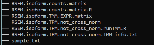
abundance_estimates_to_matrix.pl  --est_method RSEM --gene_trans_map none --name_sample_by_basedir  --cross_sample_norm TMM ../WT_REP1/RSEM.isoforms.results ../WT_REP2/RSEM.isoforms.results ../WT_REP3/RSEM.isoforms.results   ../DT_REP1/RSEM.isoforms.results ../DT_REP2/RSEM.isoforms.results ../DT_REP3/RSEM.isoforms.results

sbatch abundance.sh

RSEM

PtR (Quality Check Your Samples and Biological Replicates)

Once you’ve performed transcript quantification for each of your biological replicates, it’s good to examine the data to ensure that your biological replicates are well correlated, and also to investigate relationships among your samples. If there are any obvious discrepancies among your sample and replicate relationships such as due to accidental mis-labeling of sample replicates, or strong outliers or batch effects, you’ll want to identify them before proceeding to subsequent data analyses (such as differential expression).

cut -f 1,2 ../sample.txt >> samples_ptr.txt

nano ptr.sh

#!/bin/bash
#SBATCH --job-name=<JOB_NAME>
#SBATCH --cpus-per-task=1
#SBATCH --time=15:00
#SBATCH --mem=12g
#SBATCH --mail-type=begin
#SBATCH --mail-type=end
#SBATCH --mail-type=fail
#SBATCH --mail-user=<YOUR ID>@nevada.unr.edu
#SBATCH -o <JOB_NAME>.out # STDOUT
#SBATCH -e <JOB_NAME>.err # STDERR
#SBATCH --account=cpu-s2-bch709-1 
#SBATCH --partition=cpu-s2-core-0

PtR  --matrix RSEM.isoform.counts.matrix --samples samples_ptr.txt --CPM --log2 --min_rowSums 10  --compare_replicates

PtR  --matrix RSEM.isoform.counts.matrix --samples samples_ptr.txt --CPM  --log2 --min_rowSums 10   --sample_cor_matrix

PtR  --matrix RSEM.isoform.counts.matrix --samples samples_ptr.txt --CPM  --log2 --min_rowSums 10   --center_rows --prin_comp 3

Please transfer results to your local computer

DEG calculation

nano deseq.sh

#!/bin/bash
#SBATCH --job-name=<JOB_NAME>
#SBATCH --cpus-per-task=1
#SBATCH --time=15:00
#SBATCH --mem=12g
#SBATCH --mail-type=begin
#SBATCH --mail-type=end
#SBATCH --mail-type=fail
#SBATCH --mail-user=<YOUR ID>@nevada.unr.edu
#SBATCH -o <JOB_NAME>.out # STDOUT
#SBATCH -e <JOB_NAME>.err # STDERR
#SBATCH --account=cpu-s2-bch709-1 
#SBATCH --partition=cpu-s2-core-0


run_DE_analysis.pl --matrix RSEM.isoform.counts.matrix --samples_file samples_ptr.txt --method DESeq2 

nano edgeR.sh

#!/bin/bash
#SBATCH --job-name=<JOB_NAME>
#SBATCH --cpus-per-task=1
#SBATCH --time=15:00
#SBATCH --mem=12g
#SBATCH --mail-type=begin
#SBATCH --mail-type=end
#SBATCH --mail-type=fail
#SBATCH --mail-user=<YOUR ID>@nevada.unr.edu
#SBATCH -o <JOB_NAME>.out # STDOUT
#SBATCH -e <JOB_NAME>.err # STDERR
#SBATCH --account=cpu-s2-bch709-1 
#SBATCH --partition=cpu-s2-core-0

run_DE_analysis.pl --matrix RSEM.isoform.counts.matrix --samples_file samples_ptr.txt --method edgeR

cd DESeq2.XXXXX.dir
analyze_diff_expr.pl --matrix ../RSEM.isoform.TMM.EXPR.matrix  -P 0.001 -C 1  --samples ../samples_ptr.txt
wc -l RSEM.isoform.counts.matrix.DT_vs_WT.DESeq2.DE_results.P0.001_C1.DE.subset
cd ../

cd edgeR.XXXXX.dir
analyze_diff_expr.pl --matrix ../RSEM.isoform.TMM.EXPR.matrix  -P 0.001 -C 1  --samples ../samples_ptr.txt
wc -l RSEM.isoform.counts.matrix.DT_vs_WT.edgeR.DE_results.P0.001_C1.DE.subset

DESeq2 vs EdgeR Normalization method

DESeq and EdgeR are very similar and both assume that no genes are differentially expressed. DEseq uses a “geometric” normalisation strategy, whereas EdgeR is a weighted mean of log ratios-based method. Both normalise data initially via the calculation of size / normalisation factors.

DESeq

DESeq: This normalization method is included in the DESeq Bioconductor package (version 1.6.0) and is based on the hypothesis that most genes are not DE. A DESeq scaling factor for a given lane is computed as the median of the ratio, for each gene, of its read count over its geometric mean across all lanes. The underlying idea is that non-DE genes should have similar read counts across samples, leading to a ratio of 1. Assuming most genes are not DE, the median of this ratio for the lane provides an estimate of the correction factor that should be applied to all read counts of this lane to fulfill the hypothesis. By calling the estimateSizeFactors() and sizeFactors() functions in the DESeq Bioconductor package, this factor is computed for each lane, and raw read counts are divided by the factor associated with their sequencing lane.
DESeq2

EdgeR

Trimmed Mean of M-values (TMM): This normalization method is implemented in the edgeR Bioconductor package (version 2.4.0). It is also based on the hypothesis that most genes are not DE. The TMM factor is computed for each lane, with one lane being considered as a reference sample and the others as test samples. For each test sample, TMM is computed as the weighted mean of log ratios between this test and the reference, after exclusion of the most expressed genes and the genes with the largest log ratios. According to the hypothesis of low DE, this TMM should be close to 1. If it is not, its value provides an estimate of the correction factor that must be applied to the library sizes (and not the raw counts) in order to fulfill the hypothesis. The calcNormFactors() function in the edgeR Bioconductor package provides these scaling factors. To obtain normalized read counts, these normalization factors are re-scaled by the mean of the normalized library sizes. Normalized read counts are obtained by dividing raw read counts by these re-scaled normalization factors.
EdgeR

DESeq2 vs EdgeR Statistical tests for differential expression

DESeq2

DESeq2 uses raw counts, rather than normalized count data, and models the normalization to fit the counts within a Generalized Linear Model (GLM) of the negative binomial family with a logarithmic link. Statistical tests are then performed to assess differential expression, if any.

EdgeR

Data are normalized to account for sample size differences and variance among samples. The normalized count data are used to estimate per-gene fold changes and to perform statistical tests of whether each gene is likely to be differentially expressed.
EdgeR uses an exact test under a negative binomial distribution (Robinson and Smyth, 2008). The statistical test is related to Fisher’s exact test, though Fisher uses a different distribution.

Negative binormal

DESeq2

ϕ was assumed to be a function of μ determined by nonparametric regression. The recent version used in this paper follows a more versatile procedure. Firstly, for each transcript, an estimate of the dispersion is made, presumably using maximum likelihood. Secondly, the estimated dispersions for all transcripts are fitted to the functional form:
ϕ=a+bμ(DESeq parametric fit), using a gamma-family generalised linear model (Using regression)

EdgeR

edgeR recommends a “tagwise dispersion” function, which estimates the dispersion on a gene-by-gene basis, and implements an empirical Bayes strategy for squeezing the estimated dispersions towards the common dispersion. Under the default setting, the degree of squeezing is adjusted to suit the number of biological replicates within each condition: more biological replicates will need to borrow less information from the complete set of transcripts and require less squeezing.

DEG software comparison paper

** DEseq uses a “geometric” normalisation strategy, whereas EdgeR is a weighted mean of log ratios-based method. Both normalise data initially via the calculation of size / normalisation factors **

Draw Venn Diagram

conda create -n venn python=2.7  
conda activate venn  
conda install -c bioconda  bedtools intervene   
conda install -c r r-UpSetR r-corrplot r-Cairo  

cd ../
pwd
# /data/gpfs/assoc/bch709-1/wyim/rnaseq_slurm/DEG
mkdir Venn 
cd Venn

###DESeq2
cut -f 1 ../DEG/DESeq2.#####.dir/RSEM.isoform.counts.matrix.DT_vs_WT.DESeq2.DE_results.P0.001_C1.DT-UP.subset  | grep -v sample > DESeq.UP.subset
cut -f 1 ../DEG/DESeq2.####.dir/RSEM.isoform.counts.matrix.DT_vs_WT.DESeq2.DE_results.P0.001_C1.WT-UP.subset  | grep -v sample > DESeq.DOWN.subset

###edgeR
cut -f 1 ../DEG/edgeR.####.dir/RSEM.isoform.counts.matrix.DT_vs_WT.edgeR.DE_results.P0.001_C1.DT-UP.subset   | grep -v sample > edgeR.UP.subset
cut -f 1 ../DEG/edgeR.####.dir/RSEM.isoform.counts.matrix.DT_vs_WT.edgeR.DE_results.P0.001_C1.WT-UP.subset   | grep -v sample > edgeR.DOWN.subset


### Drawing
intervene venn -i DESeq.DOWN.subset DESeq.UP.subset edgeR.DOWN.subset edgeR.UP.subset  --type list --save-overlaps
intervene upset -i DESeq.DOWN.subset DESeq.UP.subset edgeR.DOWN.subset edgeR.UP.subset  --type list --save-overlaps
intervene pairwise  -i DESeq.DOWN.subset DESeq.UP.subset edgeR.DOWN.subset edgeR.UP.subset  --type list

BCH709 Introduction to Bioinformatics: 9_Transcriptome Assembly

Conda env

File prepare

Slurm Quick Start Tutorial

sinfo

sinfo advance

squeue

SBATCH

Important

Submit job

Trimming job running

Run trimming

squeue

Loop submission

Youtube Video for Slurm

More Slurm command

MultiQC

Running Trinity

Typical Trinity Command Line

Trinity run

Submit job

de Bruijn

python code

Please check the result

RNA-Seq reads Count Analysis

RNA-Seq reads Count Analysis job script

Job submission

Job check

Job running check

RSEM results check

Expression values and Normalization

FPKM

Reads count

Call Python

FPKM

ten to the ninth power = 10**9

TPM

Sum of FPKM

TPM calculation from FPKM

TPM calculation from reads count

Paper read

DEG calculation

Conda env

File prepare

Type sample file

Change charater to Tab

Linux command explaination

SED AWK explaination

Job file create

Run alignment

Install R-packages

abundance_estimates_to_matrix

PtR (Quality Check Your Samples and Biological Replicates)

DEG calculation

DESeq2 vs EdgeR Normalization method

DESeq

EdgeR

DESeq2 vs EdgeR Statistical tests for differential expression

DESeq2

EdgeR

Negative binormal

DESeq2

EdgeR

Draw Venn Diagram