Check your CPUs and Memory
$ lscpu
$ free
$ htop
RC file such as .bashrc, .zshrc
In Unix-like operating systems such as Linux, rc is a file name extension which stands for “run commands.” An rc file contains several statements or commands, one per line, to be executed or evaluated by the shell. Its purpose is to configure the environment and prepare the system to run specific software.
Prompt Customization for Pronghorn and Ubuntu
echo '###BCH709 ' >> ~/.bashrc

echo 'tty -s && export PS1="\[\033[38;5;164m\]\u\[$(tput sgr0)\]\[\033[38;5;15m\] \[$(tput sgr0)\]\[\033[38;5;231m\]@\[$(tput sgr0)\]\[\033[38;5;15m\] \[$(tput sgr0)\]\[\033[38;5;2m\]\h\[$(tput sgr0)\]\[\033[38;5;15m\] \[$(tput sgr0)\]\[\033[38;5;172m\]\t\[$(tput sgr0)\]\[\033[38;5;15m\] \[$(tput sgr0)\]\[\033[38;5;2m\]\w\[$(tput sgr0)\]\[\033[38;5;15m\]\n \[$(tput sgr0)\]"' >> ~/.bashrc
echo "alias ls='ls --color=auto'" >> ~/.bashrc
source ~/.bashrc
Prompt Customization for Mac
sh -c "$(curl -fsSL https://raw.github.com/ohmyzsh/ohmyzsh/master/tools/install.sh)"
source ~/.zshrc
More information is here
Linux family tree
Package Management Concepts
Contemporary distributions of Linux-based operating systems install software in pre-compiled packages, which are archives that contain binaries of software, configuration files, and information about dependencies. Furthermore, package management tools keep track of updates and upgrades so that the user doesn’t have to hunt down information about bug and security fixes.
Without package management, users must ensure that all of the required dependencies for a piece of software are installed and up-to-date, compile the software from the source code (which takes time and introduces compiler-based variations from system to system), and manage configuration for each piece of software. Without package management, application files are located in the standard locations for the system to which the developers are accustomed, regardless of which system they’re using.
Package management systems attempt to solve these problems and are the tools through which developers attempt to increase the overall quality and coherence of a Linux-based operating system. The features that most package management applications provide are:
- Package downloading: Operating-system projects provide package repositories which allow users to download their packages from a single, trusted provider. When you download from a package manager, the software can be authenticated and will remain in the repository even if the original source becomes unreliable.
- Dependency resolution: Packages contain metadata which provides information about what other files are required by each respective package. This allows applications and their dependencies to be installed with one command, and for programs to rely on common, shared libraries, reducing bulk and allowing the operating system to manage updates to the packages.
- A standard binary package format: Packages are uniformly prepared across the system to make installation easier. While some distributions share formats, compatibility issues between similarly formatted packages for different operating systems can occur.
- Common installation and configuration locations: Linux distribution developers often have conventions for how applications are configured and the layout of files in the /etc/ and /etc/init.d/ directories; by using packages, distributions are able to enforce a single standard.
- Additional system-related configuration and functionality: Occasionally, operating system developers will develop patches and helper scripts for their software which get distributed within the packages. These modifications can have a significant impact on user experience.
- Quality control: Operating-system developers use the packaging process to test and ensure that the software is stable and free of bugs that might affect product quality and that the software doesn’t cause the system to become unstable. The subjective judgments and community standards that guide packaging and package management also guide the “feel” and “stability” of a given system. In general, we recommend that you install the versions of software available in your distribution’s repository and packaged for your operating system. If packages for the application or software that you need to install aren’t available, we recommend that you find packages for your operating system, when available, before installing from source code.
The remainder of this guide will cover how to use specific package management systems and how to compile and package software yourself.
Advanced Packaging Tool (APT)
You may already be familiar with apt-get, a command which uses the advanced packaging tool to interact with the operating system’s package system. The most relevant and useful commands are (to be run with root privileges):
- ‘apt-get install package-name(s)’ - Installs the package(s) specified, along with any dependencies.
- ‘apt-get remove package-name(s)’ - Removes the package(s) specified, but does not remove dependencies.
- ‘apt-get autoremove’ - Removes any orphaned dependencies, meaning those that remain installed but are no longer required.
- ‘apt-get clean’ - Removes downloaded package files (.deb) for software that is already installed.
- ‘apt-get purge package-name(s)’ - Combines the functions of remove and clean for a specific package, as well as configuration files.
- ‘apt-get update’ - Reads the /etc/apt/sources.list file and updates the system’s database of packages available for installation. Run this after changing sources.list.
‘apt-get upgrade’ - Upgrades all packages if there are updates available. Run this after running apt-get update. While apt-get provides the most often-used functionality, APT provides additional information in the apt-cache command.
- ‘apt-cache search package-name(s)’ - If you know the name of a piece of software but apt-get install fails or points to the wrong software, this looks for other possible names.
- ‘apt-cache show package-name(s)’ - Shows dependency information, version numbers and a basic description of the package.
- ‘apt-cache depends package-name(s)’ - Lists the packages that the specified packages depends upon in a tree. These are the packages that will be installed with the apt-get install command.
- ‘apt-cache rdepends package-name(s)’ - Outputs a list of packages that depend upon the specified package. This list can often be rather long, so it is best to pipe its output through a command, like less.
- ‘apt-cache pkgnames’ - Generates a list of the currently installed packages on your system. This list is often rather long, so it is best to pipe its output through a program, like less, or direct the output to a text file. Combining most of these commands with apt-cache show can provide you with a lot of useful information about your system, the software that you might want to install, and the software that you have already installed.
Aptitude
Aptitude is another front-end interface for APT. In addition to a graphical interface, Aptitude provides a combined command-line interface for most APT functionality. Some notable commands are:
Using dpkg
Apt-get and apt-cache are merely frontend programs that provide a more usable interface and connections to repositories for the underlying package management tools called dpkg and debconf. These tools are quite powerful, and fully explaining their functionality is beyond the scope of this document. However, a basic understanding of how to use these tools is useful. Some important commands are:
- ‘dpkg -i package-file-name.deb’ - Installs a .deb file.
- ‘dpkg –list search-pattern’ - Lists packages currently installed on the system.
- ‘dpkg –configure package-name(s)’ - Runs a configuration interface to set up a package.
- ‘dpkg-reconfigure package-name(s)’ - Runs a configuration interface on an already installed package
Fedora and CentOS Package Management
Fedora and CentOS are closely related distributions, being upstream and downstream (respectively) from Red Hat Enterprise Linux (RHEL). Their main differences stem from how packages are chosen for inclusion in their repositories.
CentOS uses yum, Yellowdog Updater, Modified, as a front end to interact with system repositories and install dependencies, and also includes a lower-level tool called rpm, which allows you to interact with individual packages.
Starting with version 22, Fedora uses the dnf package manager instead of YUM to interact with rpm. DNF supports many of the same commands as YUM, with some slight changes.
Note: Many operating systems aside from RedHat use rpm packages. These include OpenSuSE, AIX, and Mandriva. While it may be possible to install an RPM packaged for one operating system on another, this is not supported or recommended, and the results of this action can vary greatly.
How about macOS?
Homebrew is package manager for Macs which makes installing lots of different software like Git, Ruby, and Node simpler. Homebrew lets you avoid possible security problems associated with using the sudo command to install software like Node. Homebrew has made extensive use of GitHub to expand the support of several packages through user contributions. In 2010, Homebrew was the third-most-forked repository on GitHub. In 2012, Homebrew had the largest number of new contributors on GitHub. In 2013, Homebrew had both the largest number of contributors and issues closed of any project on GitHub. Homebrew has spawned several sub-projects such as Linuxbrew, a Linux port now officially merged into Homebrew; Homebrew Cask, which builds upon Homebrew and focuses on the installation of GUI applications and “taps” dedicated to specific areas or programming languages like PHP.
macOS Requirements
A 64-bit Intel CPU macOS 10.12 (or higher) Command Line Tools (CLT) for Xcode A Bourne-compatible shell for installation (e.g. bash or zsh)

Install Homebrew
/usr/bin/ruby -e "$(curl -fsSL https://raw.githubusercontent.com/Homebrew/install/master/install)"
How to Update Homebrew
New versions of Homebrew come out frequently, so make sure you update it before updating any of the other software components that you’ve installed using Homebrew. * In Terminal type
brew update
How to Uninstall Homebrew
Open the Terminal app Type
ruby -e "$(curl -fsSL https://raw.githubusercontent.com/Homebrew/install/master/uninstall)This downloads and runs the uninstaller script. Follow the instructions and Homebrew will be removed from your computer.
List installed packages
We can get a list of all the installed packages on a Debian / Ubuntu server by issuing:
$ sudo dpkg --get-selections
Ubuntu server by issuing:
$ apt list --installed
on macOS
$ brew list
On RPM systems:
$ yum list installed
On BSD systems:
$ pkg_version
It is good practice to save this file as it can be useful when migrating, so we pipe it into a file:
$ dpkg --get-selections > ~/package_list
 #yum list installed
 #pkg_version
To search for a specific package run:
$ dpkg --get-selections | grep <package>
$ yum list installed "package_name"
Search packages
On Ubuntu systems:
apt search <package-name>
$ apt search firefox
$ apt search ^firefox
On macOS systems:
brew search <package-name>
$ brew search firefox
$ brew search /^firefox/
\^ means regular expressions start of the line.
Install packages
Install single packages:
On Ubuntu systems:
apt install <package-name>
On macOS systems:
brew install <package-name>
Install multiple packages:
On Ubuntu systems:
apt install <package-name> <package-name> ...
On macOS systems:
brew install <package-name> <package-name> ...
Install specific version
Search version
On Ubuntu systems:
$ apt-cache policy <package-name>
On macOS systems:
$ brew search <package-name>
Install specific version
On Ubuntu systems:
$ apt install firefox=68.0.1+build1-0ubuntu0.18.04.1
On macOS systems:
$ brew install firefox@68.0.2
Let’s install test package!
On Ubuntu systems:
$ sudo apt install screenfetch
On macOS systems:
$ /usr/bin/ruby -e "$(curl -fsSL https://raw.githubusercontent.com/Homebrew/install/master/install)"
$ brew update

$ brew install screenfetch
screenfetch
Let’s install prerequisite packages
On Ubuntu systems:
$ sudo apt-get install -y make build-essential libssl-dev zlib1g-dev libbz2-dev libreadline-dev libsqlite3-dev wget curl llvm libncurses5-dev libncursesw5-dev xz-utils tk-dev libffi-dev liblzma-dev python-openssl vim
On macOS systems:
## Install Homebrew


$ brew install openssl readline sqlite3 xz zlib
Software
| Software | Version | Manual | Available for | Description |
|---|---|---|---|---|
| FastQC | 0.11.7 | Link | Linux, MacOS, Windows | Quality control tool for high throughput sequence data. |
| HISAT2 | 2.1.0 | Link | Linux, MacOS, Windows | Mapping RNA sequences against genome |
| BWA | 0.7.17 | Link | Linux, MacOS | Mapping DNA sequences against reference genome. |
Login to HPC
You can log onto its front-end/job-submission system (pronghorn.rc.unr.edu) using your UNR NetID and password. Logging into HPC class requires an SSH client if you are >using Windows but Mac/Linux have these built into their OS. There are several available for download for the Windows platform.
ssh <YOURID>@pronghorn.rc.unr.edu
Check your CPUs and Memory
$ lscpu
$ free
$ htop
Different way to install software?
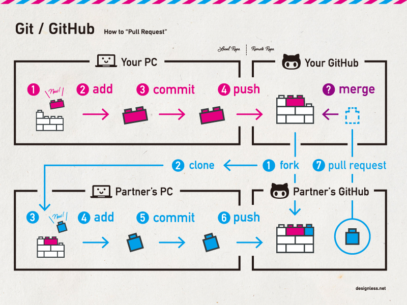
Github
What is Git and why use it?
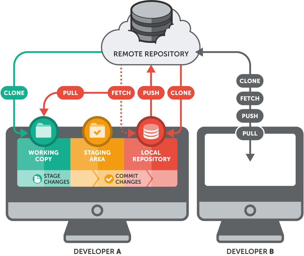
Git is an open source distributed version control system that facilitates GitHub activities on your laptop or desktop. Version control using Git is the most reasonable way to keep track of changes in code, manuscripts, presentations, and data analysis projects.
Why Version Control?
Version control is essential in creating any project that takes longer than 5 minutes to complete. Even if your memory is longer than 5 minutes, next month you are not likely to be able to retrace your steps.
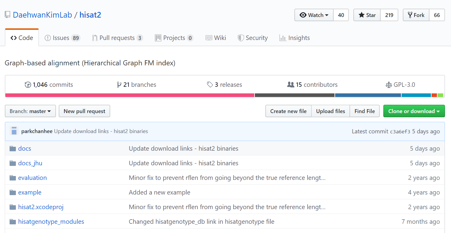
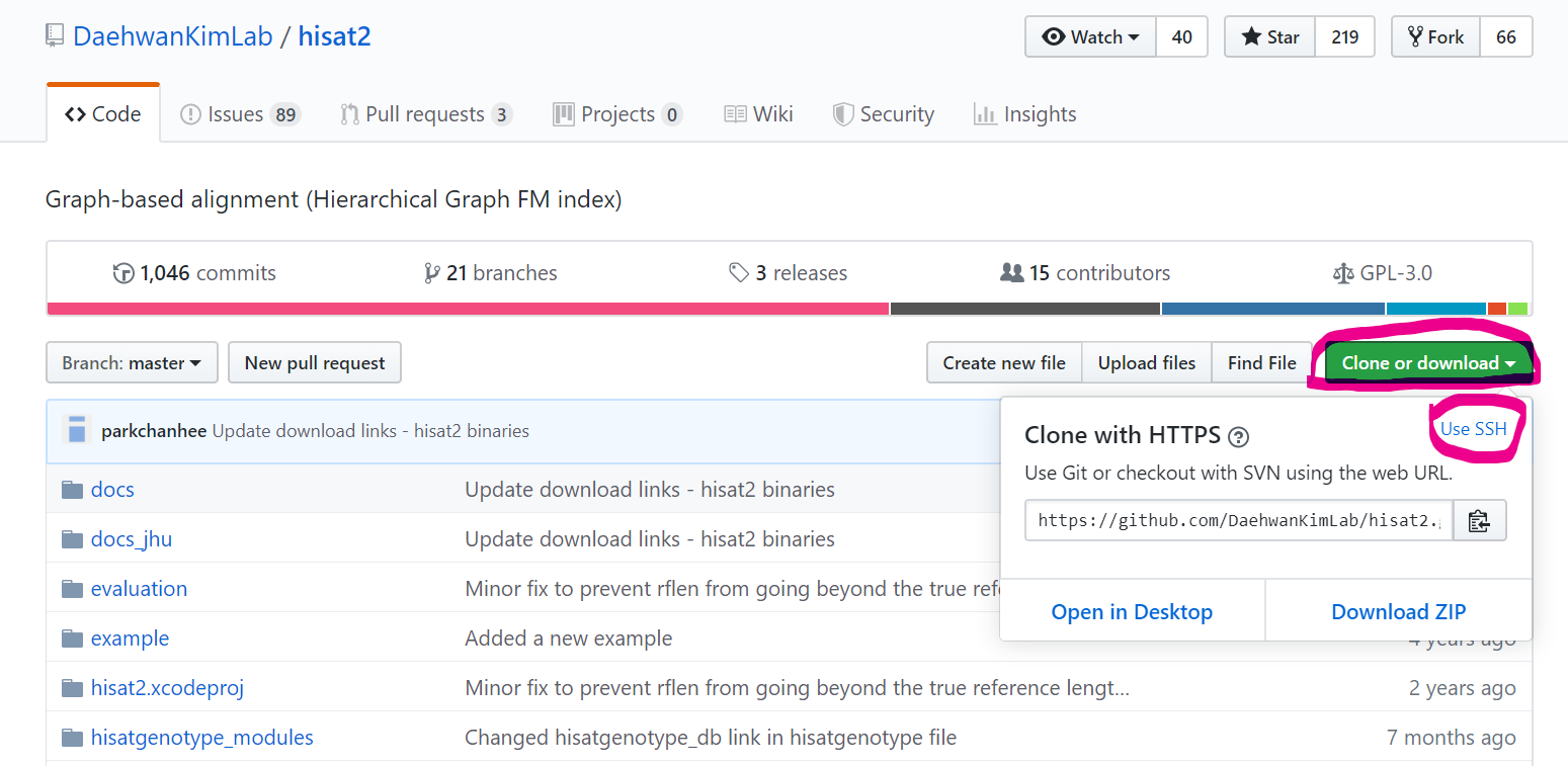
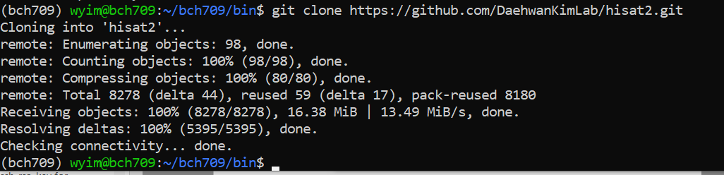
HISAT2 installation from Github
https://github.com/DaehwanKimLab/hisat2
Download
$ mkdir -p ~/bch709/bin

$ cd ~/bch709/bin

$ git clone https://github.com/DaehwanKimLab/hisat2.git

$ cd hisat2

$ ls -algh

$ less MANUAL

$ make
Conda?
-
Dependencies is one of the main reasons to use Conda. Sometimes, install a package is not as straight forward as you think. Imagine a case like this: You want to install package Matplotlib, when installing, it asks you to install Numpy, and Scipy, because Matplotlib need these Numpy and Scipy to work. They are called the dependencies of Matplotlib. For Numpy and Scipy, they may have their own dependencies. These require even more packages.
-
Conda provide a solution for this situation: when you install package Matplotlib, it will automatically install all the dependencies like Numpy and Scipy. So you don’t have to install them one by one, manually. This can save you great amount of time.
-
The other advantage of conda, is that conda can have multiple environments for different projects. As mentioned at the very beginning, it can have two separate environments of different versions of software. Using conda environment on BioHPC
Installing Packages Using Conda
Conda is a package manager, which helps you find and install packages such as numpy or scipy. It also serves as an environment manager, and allows you to have multiple isolated environments for different projects on a single machine. Each environment has its own installation directories, that doesn’t share packages with other environments.
For example, you need python 2.7 and Biopython 1.60 in project A, while you also work on another project B, which needs python 3.5 and Biopython 1.68. You can use conda to create two separate environments for each project, and you can switch between different versions of packages easily to run your project code.
Anaconda or Miniconda?
-
Anaconda includes both Python and conda, and additionally bundles a suite of other pre-installed packages geared toward scientific computing. Because of the size of this bundle, expect the installation to consume several gigabytes of disk space.
-
Miniconda gives you the Python interpreter itself, along with a command-line tool called conda which operates as a cross-platform package manager geared toward Python packages, similar in spirit to the apt or yum tools that Linux users might be familiar with.
Miniconda3
Miniconda is a package manager that simplifies the installation process. Please first install miniconda3 (installation instructions below), and then proceed to the installation of individual tools.
Install Miniconda
Visit the miniconda page and get ready to download the installer of your choice/system.
There are several different env in this world.
https://repo.anaconda.com/miniconda/
Linux
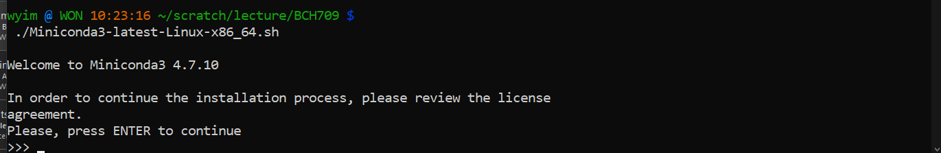
To install miniconda3, type:
$ curl -O https://repo.anaconda.com/miniconda/Miniconda3-latest-Linux-x86_64.sh
$ bash Miniconda3-latest-Linux-x86_64.sh
Then, follow the instructions that you are prompted with on the screen to install Miniconda3.

MacOS
To install miniconda3, type:
$ curl -O https://repo.anaconda.com/miniconda/Miniconda3-latest-MacOSX-x86_64.sh
$ bash Miniconda3-latest-MacOSX-x86_64.sh
Then, follow the instructions that you are prompted with on the screen to install Miniconda3.
Reload your Conda enviroment
Linux
$ source ~/.bashrc
Mac OS
$ source ~/.bash_profile
$ source ~/.zshrc
Initialize Miniconda3
$ conda init
Create new conda environment
Create a conda environment named test with latest anaconda package.
$ conda create -n bch709
Alternatively you can specify python version
$ conda create -n snowdeer_env python=2.7.16
*Usually, the conda environment is installed in your home directory on computer, /home/<your username>. The newly created environment
Use the environment you just created
Activate your environment:
$ conda activate bch709
It will show your environment name at the beginning of the prompt.

Install packages in the conda environment
Install from default conda channel You can search if your package is in the default source from Anaconda collection. Besides the 200 pre-built Anaconda packages, it contains over 600 extra scientific and analytic packages. All the dependencies will also be installed automatically.
$ conda search <package>
$ conda install <package>
Install from conda-forge channel (example: hisat2)
Conda channels are the remote repository that conda takes to search or download the packages. If you want to install a package that is not in the default Anaconda channel, you can tell conda which channel containing the package, so that conda can find and install. Conda-forge is a GitHub community-led conda channel, containing general packages which are not in the default Anaconda source. All the packages from conda-forge is listed at https://bioconda.github.io/conda-recipe_index.html
$ conda search hisat2
$ conda search -c bioconda hisat2
Install from bioconda channel (example: hisat2)
Bioconda is another channel of conda, focusing on bioinformatics software. Instead of adding “-c” to search a channel only one time, “add channels” tells Conda to always search in this channel, so you don’t need to specify the channel every time. Remember to add channel in this order, so that Bioconda channel has the highest priority. Channel orders will be explained in next part.
Adding channels will not generate any command line output. Then, you can install Stringtie from the Bioconda channel
$ conda install -c bioconda hisat2
![]()
Install R and R packages
The Conda package manager is not limited to Python. R and R packages are well supported by a conda channel maintained by the developers of Conda. The R-essentials include all the popular R packages with all of their dependencies. The command below opens R channel by “-c r”, and then install the r-essentials using R channel.
$ conda install -c r r-essentials
Update R packages
$ conda update -c r r-essentials
$ conda update -c r r-<package name>
More conda commands:.
search packages
This will search the packages in conda
$ conda search hisat2
See all available environments
You can check the list of all separate environments, and it will show * at your current environment. In the figure below, it shows root, since I’m not in any conda environment.
$ conda env list
List all package installed
This will show all the packages and versions you’ve installed.
$ conda list
Update packages or conda itself
This will update to the newest version of one package, or conda itself. update package
$ conda update <package>
update package in env
conda update --name <ENV_name> <package>
update conda itself
$ conda update -n test --all
$ conda update -n bch709 --all
Uninstall package from the environment
$ conda uninstall <package name>
Exit current environment:
You can exit, when you finish your work in the current environment.
$ conda deactivate
Remove environment
$ conda env remove --name bch709
When you finish your project, you might want to remove the environment. However, it is not recommended because you might want to update some work in this project in the future.
Enviroment export
conda env export --name <ENVIRONMENT> --file <outputfilename>.yaml
Envrioment import
conda env create --file <outputfilename>.yaml
HPC clusters
This exercise mainly deals with using HPC clusters for large scale data (Next Generation Sequencing analysis, Genome annotation, evolutionary studies etc.). These clusters have several processors with large amounts of RAM (compared to typical desktop/laptop), which makes it ideal for running programs that are computationally intensive. The operating system of these clusters are primarily UNIX and are mainly operated via command line. All the commands that you have learned in the previous exercises can be used on HPC.
Pronghorn High Performance Computing offers shared cluster computing infrastructure for researchers and students at UNR. Brief descriptions for the available resources can be found here: https://www.unr.edu/research-computing/hpc. To begin with, you need to request permission for accessing these resources either through your department or through your advisor. All workshop attendees will have their account setup on HPC class education cluster and they can use their UNR NetID and the password for logging-in. You should have already received a confirmation email about your account creation with instructions on how to connect to the cluster. In this exercise we will specifically teach you how to connect to a remote server (HPC), transfer files in and out of the server, and running programs by requesting resources.
You can log onto its front-end/job-submission system (pronghorn.rc.unr.edu) using your UNR NetID and password. Logging into HPC class requires an SSH client if you are >using Windows but Mac/Linux have these built into their OS. There are several available for download for the Windows platform.
ssh <YOURID>@pronghorn.rc.unr.edu
There are a number of ways to transfer data to and from HPC clusters. Which you should use depends on several factors, including the ease of use for you personally, connection speed and bandwidth, and the size and number of files which you intend to transfer. Most common options include scp, rsync (command line) and SCP and SFTP clients (GUI). scp (secure copy) is a simple way of transferring files between two machines that use the SSH (Secure SHell) protocol. You may use scp to connect to any system where you have SSH (login) access. scp is available as a protocol choice in some graphical file transfer programs and also as a command line program on most Linux, UNIX, and Mac OS X systems. scp can copy single files, but will also recursively copy directory contents if given a directory name. scp can be used as follows:
- to a remote system from local
scp sourcefile username@pronghorn.rc.unr.edu:somedirectory/ - from a remote system to local
scp username@pronghorn.rc.unr.edu:somedirectory/sourcefile destinationfile - recursive directory copy to a remote system from local
scp -r SourceDirectory/ username@pronghorn.rc.unr.edu:somedirectory/<!–
rsync is a fast and extraordinarily versatile file copying tool. It can synchronize file trees across local disks, directories or across a network
- Synchronize a local directory with the remote server directory
rsync -avhP path/to/SourceDirectory username@pronghorn.rc.unr.edu:somedirectory/ - Synchronize a remote directory with the local directory
rsync -avhP username@hpronghorn.rc.unr.edu:SourceDirectory/ path/to/Destination/–>
Paper reading
Please read this paper https://genomebiology.biomedcentral.com/articles/10.1186/s13059-016-0881-8
RNA Sequencing

- The transcriptome is spatially and temporally dynamic
- Data comes from functional units (coding regions)
- Only a tiny fraction of the genome
Introduction
Sequence based assays of transcriptomes (RNA-seq) are in wide use because of their favorable properties for quantification, transcript discovery and splice isoform identification, as well as adaptability for numerous more specialized measurements. RNA-Seq studies present some challenges that are shared with prior methods such as microarrays and SAGE tagging, and they also present new ones that are specific to high-throughput sequencing platforms and the data they produce. This document is part of an ongoing effort to provide the community with standards and guidelines that will be updated as RNASeq matures and to highlight unmet challenges. The intent is to revise this document periodically to capture new advances and increasingly consolidate standards and best practices.
RNA-Seq experiments are diverse in their aims and design goals, currently including multiple types of RNA isolated from whole cells or from specific sub-cellular compartments or biochemical classes, such as total polyA+ RNA, polysomal RNA, nuclear ribosome-depleted RNA, various size fractions of RNA and a host of others. The goals of individual experiments range from major transcriptome “discovery” that seeks to define and quantify all RNA species in a starting RNA sample to experiments that simply need to detect significant changes in the more abundant RNA classes across many samples.

Seven stages to data science
- Define the question of interest
- Get the data
- Clean the data
- Explore the data
- Fit statistical models
- Communicate the results
- Make your analysis reproducible
What do we need to prepare ?
Sample Information
a. What kind of material it is should be noted: Tissue, cell line, primary cell type, etc… b. It’s ontology term (a DCC wrangler will work with you to obtain this) c. If any treatments or genetic modifications (TALENs, CRISPR, etc…) were done to the sample prior to RNA isolation. d. If it’s a subcellular fraction or derived from another sample. If derived from another sample, that relationship should be noted. e. Some sense of sample abundance: RNA-Seq data from “bulk” vs. 10,000 cell equivalents can give very different results, with lower input samples typically being less reproducible. Having a sense of the amount of starting material here is useful. f. If you received a batch of primary or immortalized cells, the lot #, cat # and supplier should be noted. g. If cells were cultured out, the protocol and methods used to propagate the cells should be noted. h. If any cell phenotyping or other characterizations were done to confirm it’s identify, purity, etc.. those methods should be noted.
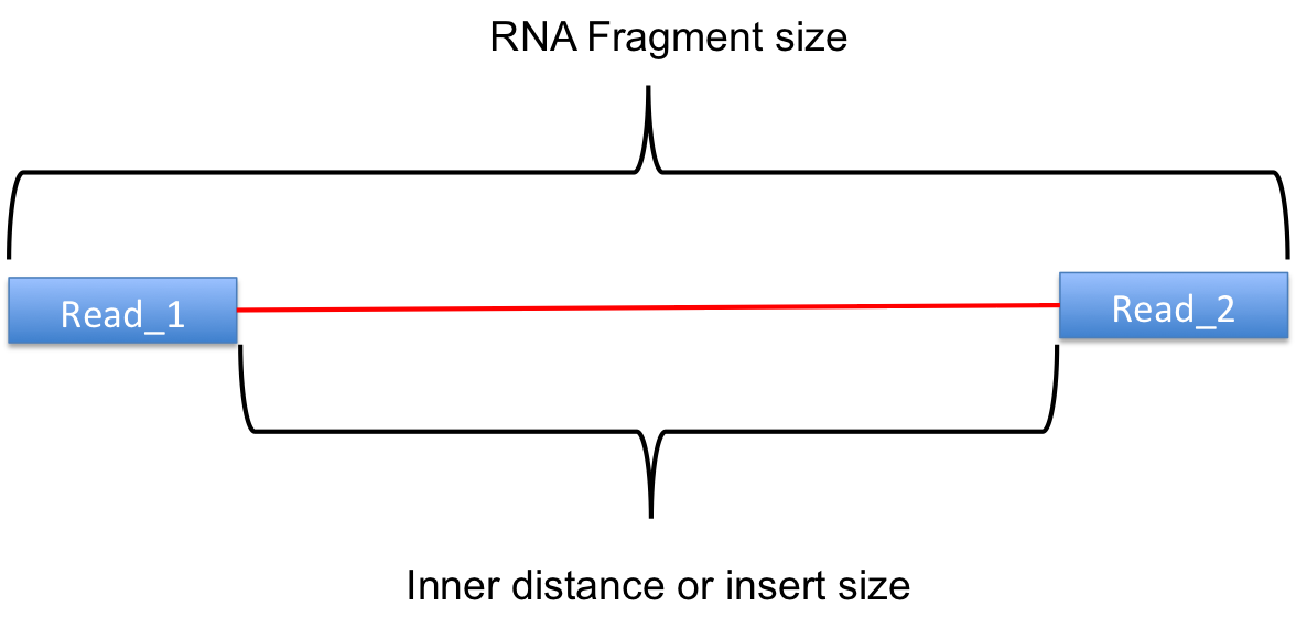
RNA Information:
RNAs come in all shapes and sizes. Some of the key properties to report are: a. Total RNA, Poly-A(+) RNA, Poly-A(-) RNA b. Size of the RNA fraction: we typically have a + 200 and – 200 cutoff, but there is a wide range, i.e. microRNA-sized, etc… c. If the RNA was treated with Ribosomal RNA depletion kits (RiboMinus, RiboZero): please note the kit used.
Protocols:
There are several methods used to isolate RNAs with that work fine for the purposes of RNA-Seq. For all the ENCODE libraries that we make, we provide a document that lists in detail: a. The RNA isolation methods, b. Methods of size selections c. Methods of rRNA removal d. Methods of oligo-dT selections e. Methods of DNAse I treatments
Experimental Design
- Balanced design
- Technical replicates not necessary (Marioni et al., 2008)
- Biological replicates: 6 - 12 (Schurch et al., 2016)
- Power analysis
Reading materials
Paul L. Auer and R. W. Doerge “Statistical Design and Analysis of RNA Sequencing Data” Genetics June 1, 2010 vol. 185 no.2 405-416 Busby, Michele A., et al. “Scotty: a web tool for designing RNA-Seq experiments to measure differential gene expression.” Bioinformatics 29.5 (2013): 656-657 Marioni, John C., et al. “RNA-seq: an assessment of technical reproducibility and comparison with gene expression arrays.” Genome research (2008) Schurch, Nicholas J., et al. “How many biological replicates are needed in an RNA-seq experiment and which differential expression tool should you use?.” Rna (2016) Zhao, Shilin, et al. “RnaSeqSampleSize: real data based sample size estimation for RNA sequencing.” BMC bioinformatics 19.1 (2018): 191
Replicate number
In all cases, experiments should be performed with two or more biological replicates, unless there is a compelling reason why this is impractical or wasteful (e.g. overlapping time points with high temporal resolution). A biological replicate is defined as an independent growth of cells/tissue and subsequent analysis. Technical replicates from the same RNA library are not required, except to evaluate cases where biological variability is abnormally high. In such instances, separating technical and biological variation is critical. In general, detecting and quantifying low prevalence RNAs is inherently more variable than high abundance RNAs. As part of the ENCODE pipeline, annotated transcript and genes are quantified using RSEM and the values are made available for downstream correlation analysis. Replicate concordance: the gene level quantification should have a Spearman correlation of >0.9 between isogenic replicates and >0.8 between anisogenic replicates.
RNA extraction
- Sample processing and storage
- Total RNA/mRNA/small RNA
- DNAse treatment
- Quantity & quality
- RIN values (Strong effect)
- Batch effect
- Extraction method bias (GC bias)
Reading materials
Romero, Irene Gallego, et al. “RNA-seq: impact of RNA degradation on transcript quantification.” BMC biology 12.1 (2014): 42
Kim, Young-Kook, et al. “Short structured RNAs with low GC content are selectively lost during extraction from a small number of cells.” Molecular cell 46.6 (2012): 893-89500481-9).
RNA Quantification and Quality Control: When working with bulk samples, throughout the various steps we periodically assess the quality and quantity of the RNA. This is typically done on a BioAnalyzer. Points to check are: a. Total RNA b. After oligo-dT size selections c. After rRNA-depletions d. After library construction
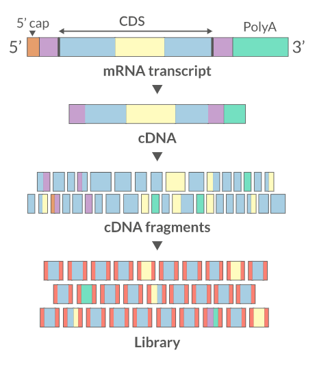
Library prep
- PolyA selection
- rRNA depletion
- Size selection
- PCR amplification (See section PCR duplicates)
- Stranded (directional) libraries
- Accurately identify sense/antisense transcript
- Resolve overlapping genes
- Exome capture
- Library normalisation
- Batch effect
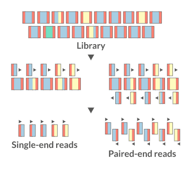
Sequencing:
There are several sequencing platforms and technologies out there being used. It is important to provide the following pieces of information: a. Platform: Illumina, PacBio, Oxford Nanopore, etc… b. Format: Single-end, Pair-end, c. Read Length: 101 bases, 125 bases, etc… d. Unusual barcode placement and sequence: Some protocols introduce barcodes in noncustomary places. If you are going to deliver a FASTQ file that will contain the barcode sequences in it or other molecular markers – you will need to report both the position in the read(s) where they are and their sequence(s). e. Please provide the sequence of any custom primers that were used to sequence the library
Sequencing depth.
The amount of sequencing needed for a given sample is determined by the goals of the experiment and
the nature of the RNA sample. Experiments whose purpose is to evaluate the similarity between the
transcriptional profiles of two polyA+ samples may require only modest depths of sequencing.
Experiments whose purpose is discovery of novel transcribed elements and strong quantification of
known transcript isoforms requires more extensive sequencing.
• Each Long RNA-Seq library must have a minimum of 30 million aligned reads/mate-pairs.
• Each RAMPAGE library must have a minimum of 20 million aligned reads/mate-pairs.
• Each small RNA-Seq library must have a minimum of 30 million aligned reads/mate-pairs.
Quantitative Standards (spike-ins).
It is highly desirable to include a ladder of RNA spike-ins to calibrate quantification, sensitivity, coverage and linearity. Information about the spikes should include the stage of sample preparation that the spiked controls were added, as the point of entry affects use of spike data in the output. In general, introducing spike-ins as early in the process as possible is the goal, with more elaborate uses of different spikes at different steps being optional (e.g. before poly A+ selection, at the time of cDNA synthesis, or just prior to sequencing). Different spike-in controls are needed for each of the RNA types being analyzed (e.g. long RNAs require different quantitative controls from short RNAs). Such standards are not yet available for all RNA types. Information about quantified standards should also include: a) A FASTA (or other standard format) file containing the sequences of each spike in. b) Source of the spike-ins (home-made, Ambion, etc..) c) The concentration of each of the spike-ins in the pool used.
Hong et al., 2016, Principles of metadata organization at the ENCODE data coordination center.
QC FAIL?
https://sequencing.qcfail.com/
Fastq format
FASTQ format is a text-based format for storing both a biological sequence (usually nucleotide sequence) and its corresponding quality scores.
The format is similar to fasta though there are differences in syntax as well as integration of quality scores. Each sequence requires at least 4 lines:
- The first line is the sequence header which starts with an ‘@’ (not a ‘>’!). Everything from the leading ‘@’ to the first whitespace character is considered the sequence identifier. Everything after the first space is considered the sequence description
- The second line is the sequence.
- The third line starts with ‘+’ and can have the same sequence identifier appended (but usually doesn’t anymore).
- The fourth line are the quality scores
The FastQ sequence identifier generally adheres to a particular format, all of which is information related to the sequencer and its position on the flowcell. The sequence description also follows a particular format and holds information regarding sample information.
$ pwd

$ cd ~/

$ mkdir bch709/rnaseq

$ cd bch709/rnaseq/

$ pwd

$ ls /data/gpfs/assoc/bch709-4/data/

$ cp /data/gpfs/assoc/bch709-4/data/*.gz .

$ ls -algh

$ zcat paired2.fastq.gz | head
@A00261:180:HL7GCDSXX:2:1101:30572:1047/2
AAAATACATTGATGACCATCTAAAGTCTACGGCGTATGCGACTGATGAAGTATATTGCACCACCTGAGGGTGATGCTAATACTACTGTTGACGATAATGCTGATCTTCTTGCTAAGCTTAATATTGTTGGTGTTGAACCTAATGTTGGTG
+
FFFFFFFFFFFFFFFFFFFFFFFFFFFFFFFFFFFFFFFFFFFFFFFFFFFFFFFFFFFFFFFFFFFFFFFFFFFFFFFFFFFFF:FFFFFFFFFFFFFFFFFFFFFFFFFFFFFFFFFFFFFFFFFFFFFFFFFFFFFF:FFFFFFFFF
@A00261:180:HL7GCDSXX:2:1101:21088:1094/2
ATCTCACATCGTTCCCTCAAGATTCTGAATTTTGGCAGCTCATTGCATTCTGTGCCGGCACTGGTGGTTCGATGCTTGTCATTGGTTCTGCTGCTGGTGTAGCCTTCATGGGGATGGAGAAAGTCGATTTCTTTTGGTATTTCCGAAAGG
+
FFFFFFFFFFFFFFFFFFFFFF:FFFFFFFFFFFFFFFFFFFFFFFFFFFFFFFFFFFFFFFFFFFF:FFFFFFFF:FFFFFFFFFFFFFFFFFFFFFFFFFFFFF:FFFFFFFFFFFFFFFFFFFFFFFFFFFFFFFFFFFFFFFFFFF
@A00261:180:HL7GCDSXX:2:1101:21251:1125/2
CGGTGGAAAAGGAAACAGCTTTGGAAGGTTGATTCCATTACAGATTCGATTCGAAACTATGGTTCAGATTTCCGATCTTCCACGGGATTTGACAGAGGAGGTGCTCTCTAGGATTCCGGTGACATCTATGAGAGCAGTGAGATTTACTTG
- A00261 : Instrument name
- 180 : run ID
- HL7GCDSXX : Flowcell ID
- 2 : Flowcell lane
- 1101 : tile number within the flowcell lane
- 30572 : X-coordinate of the cluster within tile
- 1047 : Y-coordinate of the cluster within tile
- /2 : member of a pair 1 or 2 (Paired end reads only)
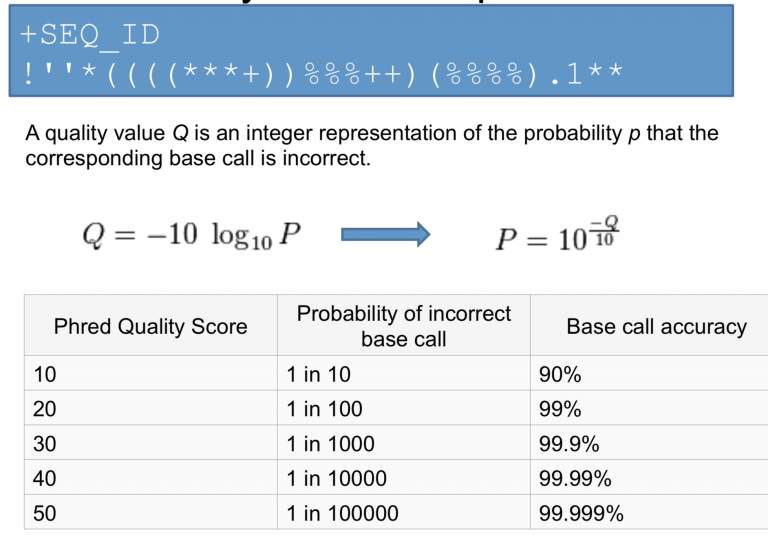
Quality Scores
Quality scores are a way to assign confidence to a particular base within a read. Some sequencers have their own proprietary quality encoding but most have adopted Phred-33 encoding. Each quality score represents the probability of an incorrect basecall at that position.
Phred Quality Score Encoding
Quality scores started as numbers (0-40) but have since changed to an ASCII encoding to reduce filesize and make working with this format a bit easier, however they still hold the same information. ASCII codes are assigned based on the formula found below. This table can serve as a lookup as you progress through your analysis.
Quality Score Interpretation
Once you know what each quality score represents you can then use this chart to understand the confidence in a particular base.
Conda enviroment
$ conda create -n rnaseq_test python=3 -c bioconda multiqc fastqc trim-galore hisat2 bc


$ conda activate rnaseq_test
Reads QC
- Number of reads
- Per base sequence quality
- Per sequence quality score
- Per base sequence content
- Per sequence GC content
- Per base N content
- Sequence length distribution
- Sequence duplication levels
- Overrepresented sequences
- Adapter content
- Kmer content
$ conda search fastqc
$ conda install -c bioconda fastqc
Run fastqc
$ fastqc --help
$ fastqc -t <YOUR CPU COUNT> paired1.fastq.gz  paired2.fastq.gz
How to make a report?
$ conda search multiqc
$
$ conda install -c bioconda multiqc
$ multiqc --help
$ multiqc .
$ cp -r multiqc* <YOUR DESKTOP FOLDER>
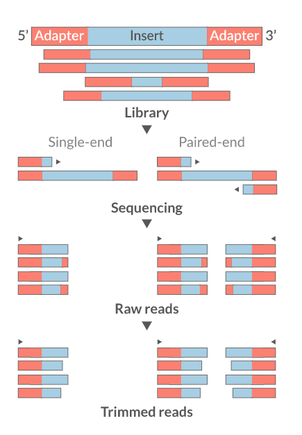
Trim the reads
- Trim IF necessary
- Synthetic bases can be an issue for SNP calling
- Insert size distribution may be more important for assemblers
- Trim/Clip/Filter reads
- Remove adapter sequences
- Trim reads by quality
- Sliding window trimming
- Filter by min/max read length
- Remove reads less than ~18nt
- Demultiplexing/Splitting
Cutadapt
fastp
Skewer
Prinseq
Trimmomatics
Trim Galore
Install Trim Galore
$ conda install -c bioconda trim-galore
Run trimming
$ trim_galore --help

$ trim_galore --paired   --three_prime_clip_R1 5 --three_prime_clip_R2 5 --cores 2  --max_n 40  --fastqc --gzip -o trim paired1.fastq.gz paired2.fastq.gz

$ multiqc .
Align the reads (mapping)
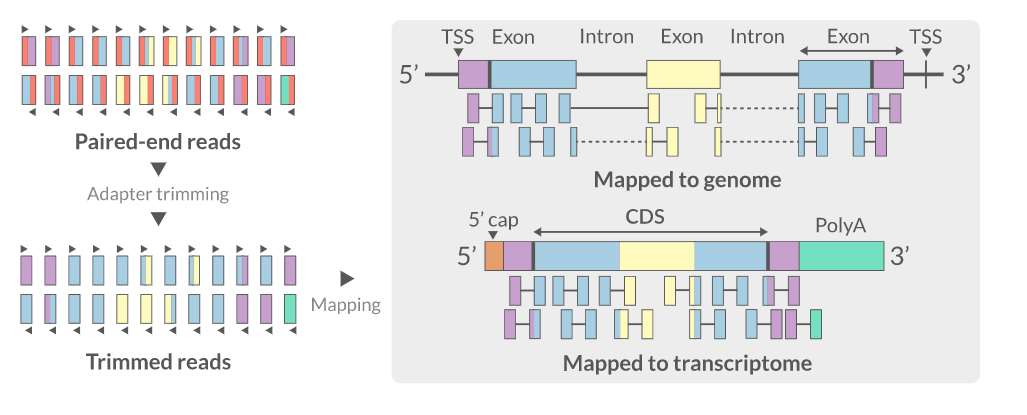
- Aligning reads back to a reference sequence
- Mapping to genome vs transcriptome
- Splice-aware alignment (genome)
STAR
HISAT2
GSNAP
Bowtie2
Novoalign
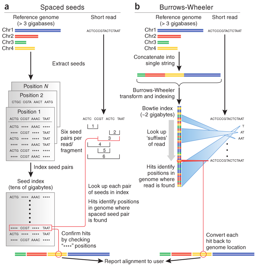
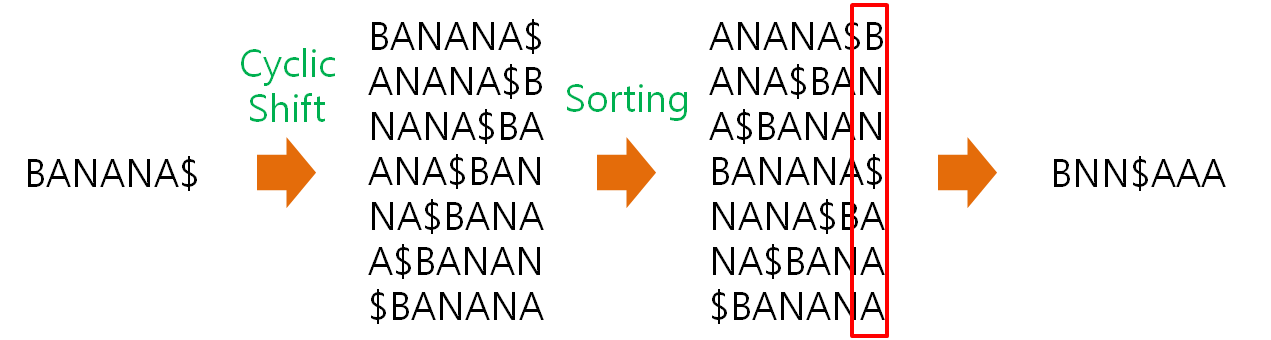
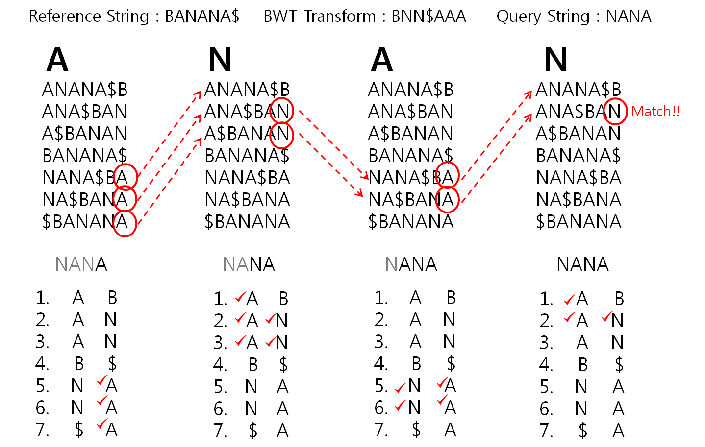
Install HISAT2 (graph FM index, spin off version Burrows-Wheeler Transform)
$ conda install -c bioconda hisat2
Download reference sequence
$ cp /data/gpfs/assoc/bch709-4/data/bch709.fasta .
HISAT2 indexing
$ hisat2-build --help
$ hisat2-build bch709.fasta bch709
HISAT2 mapping
$ hisat2 -x bch709 --threads <YOUR CPU COUNT> -1 trim/paired1_val_1.fq.gz -2 trim/paired2_val_2.fq.gz -S align.sam
SAM file format
Check result
$ head align.sam
SAM file
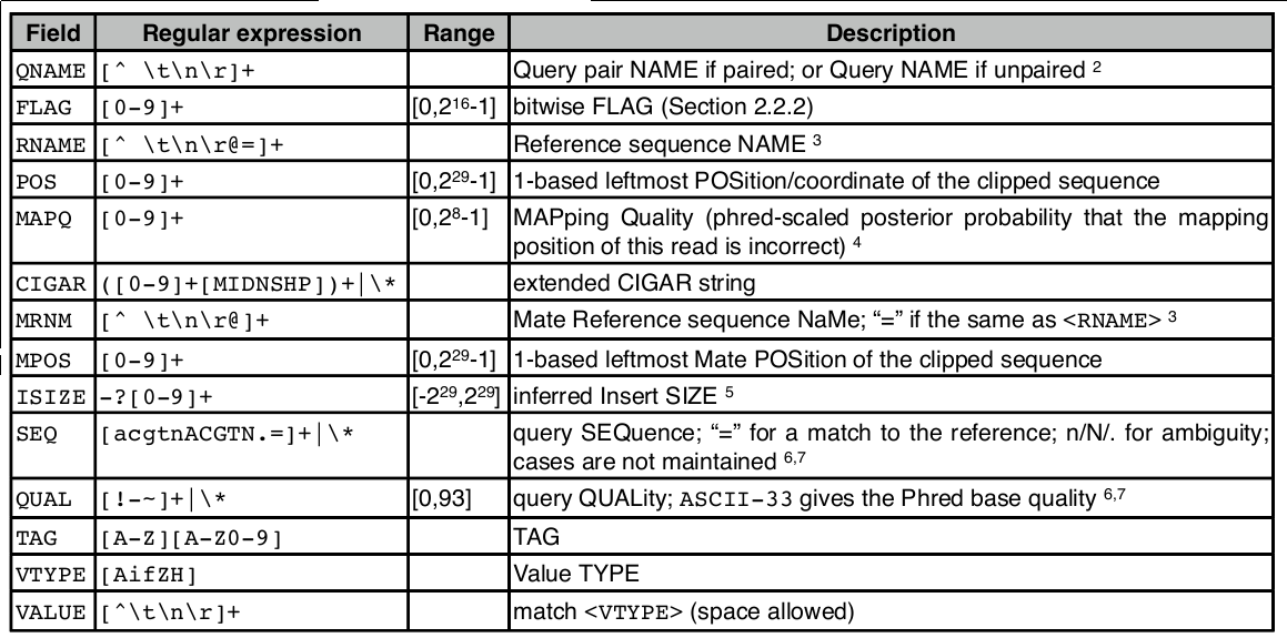
<QNAME> <FLAG> <RNAME> <POS> <MAPQ> <CIGAR> <MRNM> <MPOS> <ISIZE> <SEQ> <QUAL> [<TAG>:<VTYPE>:<VALUE> [...]]
SAM flag
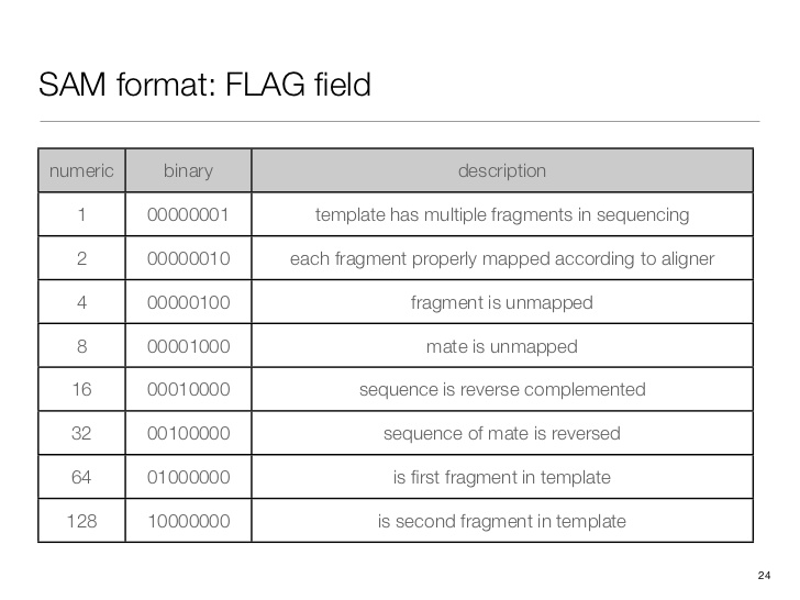
Demical to binary
$ echo 'obase=163;10' | bc
If you don’t have bc, please install through conda
$ conda install bc
SAM tag
There are a bunch of predefined tags, please see the SAM manual for more information. For the tags used in this example:
Any tags that start with X? are reserved fields for end users: XT:A:M, XN:i:2, XM:i:0, XO:i:0, XG:i:0
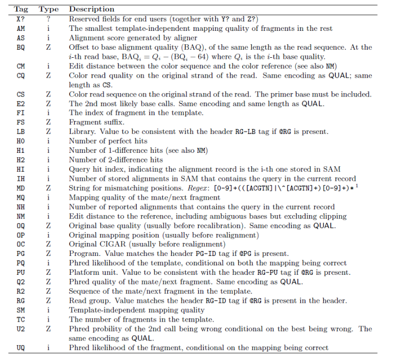
More information is below.
http://samtools.github.io/hts-specs/
SAMtools
SAM (Sequence Alignment/Map) format is a generic format for storing large nucleotide sequence alignments. SAM aims to be a format that:
- Is flexible enough to store all the alignment information generated by various alignment programs;
- Is simple enough to be easily generated by alignment programs or converted from existing alignment formats;
- Is compact in file size;
- Allows most of operations on the alignment to work on a stream without loading the whole alignment into memory;
- Allows the file to be indexed by genomic position to efficiently retrieve all reads aligning to a locus.
SAM Tools provide various utilities for manipulating alignments in the SAM format, including sorting, merging, indexing and generating alignments in a per-position format. http://samtools.sourceforge.net/
$ conda install -c bioconda samtools
$ samtools view -Sb align.sam > align.bam
$ samtools sort align.bam  align_sort
$ samtools index align_sort.bam
BAM file
A BAM file (.bam) is the binary version of a SAM file. A SAM file (.sam) is a tab-delimited text file that contains sequence alignment data.
| SAM/BAM | size |
|---|---|
| align.sam | 903M |
| align.bam | 166M |
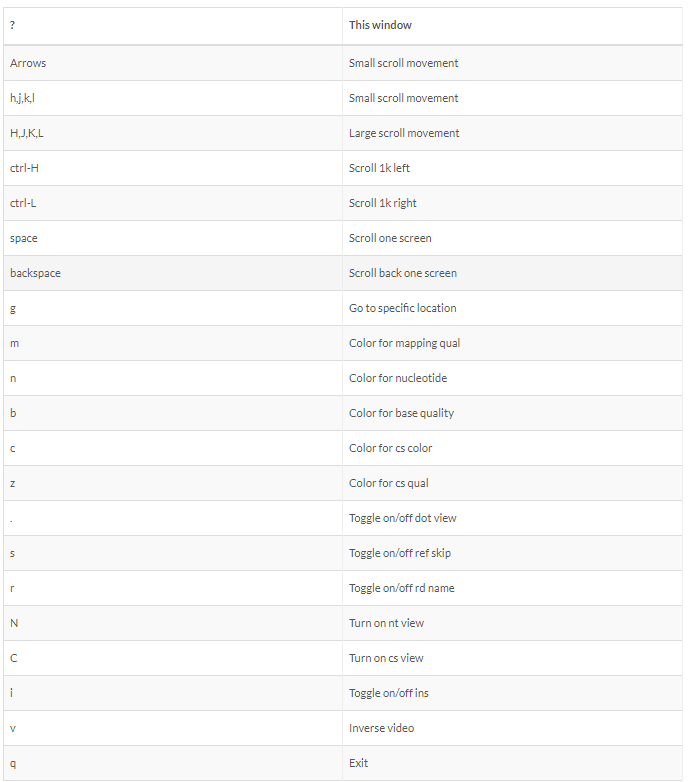
Alignment visualization
samtools tview align_sort.bam bch709.fasta
Alignment QC
- Number of reads mapped/unmapped/paired etc
- Uniquely mapped
- Insert size distribution
- Coverage
- Gene body coverage
- Biotype counts / Chromosome counts
- Counts by region: gene/intron/non-genic
- Sequencing saturation
- Strand specificity
samtools > stats
bamtools > stats
QoRTs
RSeQC
Qualimap
Quantification • Counts
- Read counts = gene expression
- Reads can be quantified on any feature (gene, transcript, exon etc)
- Intersection on gene models
- Gene/Transcript level
featureCounts HTSeq RSEM Cufflinks Rcount
conda install -c bioconda subread
conda install -c bioconda rsem
Quantification method
- PCR duplicates
- Ignore for RNA-Seq data
- Computational deduplication (Don’t!)
- Use PCR-free library-prep kits
-
Use UMIs during library-prep
- Multi-mapping
- Added (BEDTools multicov)
- Discard (featureCounts, HTSeq)
- Distribute counts (Cufflinks)
- Rescue
- Probabilistic assignment (Rcount, Cufflinks)
- Prioritise features (Rcount)
- Probabilistic assignment with EM (RSEM)
Reference
Fu, Yu, et al. “Elimination of PCR duplicates in RNA-seq and small RNA-seq using unique molecular identifiers.” BMC genomics 19.1 (2018): 531 Parekh, Swati, et al. “The impact of amplification on differential expression analyses by RNA-seq.” Scientific reports 6 (2016): 25533 Klepikova, Anna V., et al. “Effect of method of deduplication on estimation of differential gene expression using RNA-seq.” PeerJ 5 (2017): e3091
Differential expression
DESeq2 edgeR (Neg-binom > GLM > Test) Limma-Voom (Neg-binom > Voom-transform > LM > Test)
conda install -c bioconda bioconductor-deseq2
Functional analysis • GO
Gene enrichment analysis (Hypergeometric test) Gene set enrichment analysis (GSEA) Gene ontology / Reactome databases
Conda deactivate
$ conda deactivate
$ conda env remove --name rnaseq
Reading material
Conesa, Ana, et al. “A survey of best practices for RNA-seq data analysis.” Genome biology 17.1 (2016): 13
Reference:
- Conda documentation https://docs.conda.io/en/latest/
- Conda-forge https://conda-forge.github.io/
- BioConda https://bioconda.github.io/