Env setting
conda create -n preprocessing python=3 -y

conda activate preprocessing

conda install  -c r -c conda-forge -c anaconda -c bioconda  trim-galore jellyfish=2.2.10 'multiqc<1.34' nanostat nanoplot -y
conda create -n genomeassembly -y
conda activate genomeassembly
conda install -c conda-forge -c anaconda -c bioconda spades canu pacbio_falcon samtools minimap2 'multiqc<1.34' assembly-stats openssl=1.0 -y
conda install  -c r -c conda-forge -c anaconda -c bioconda  r-ggplot2 r-stringr r-scales r-argparse -y
Genome assembly
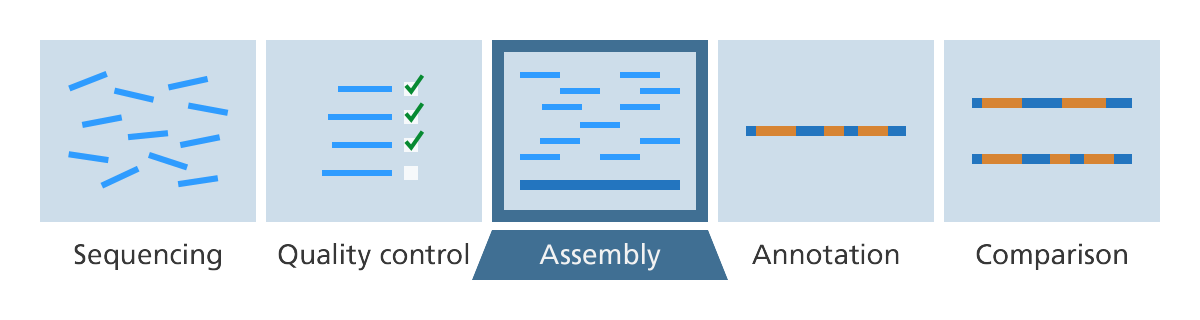
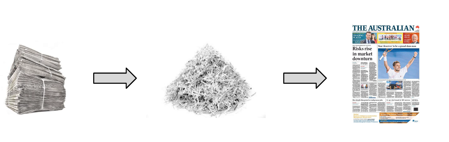
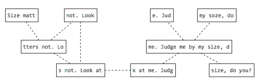
After DNA sequencing is complete, the fragments of DNA that come out of the machine are all jumbled up. Like a jigsaw puzzle we need to take the pieces of the genome and put them back together.
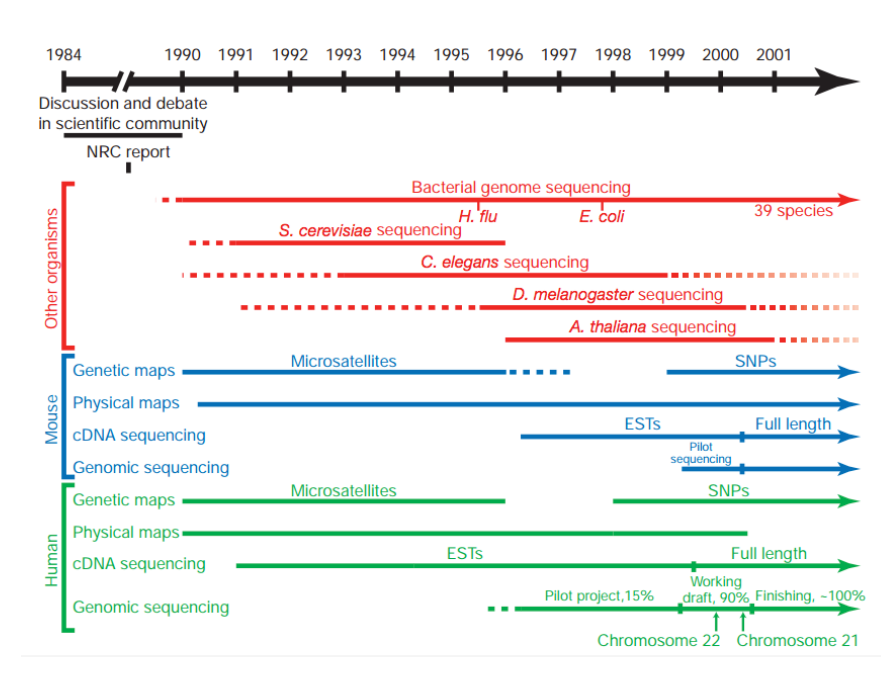
The human genome required a significant technological push
25✕ larger than any previously sequenced genome
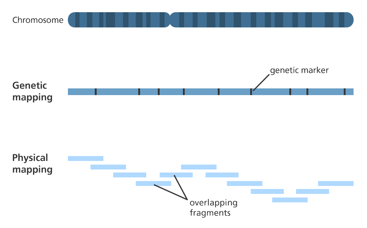
- Construction of genetic and physical maps of human and mouse genomes
- Sequencing of yeast and worm genomes
- Pilot projects to test the feasibility and cost effectiveness of large-scale sequencing
What’s the challenge?
-
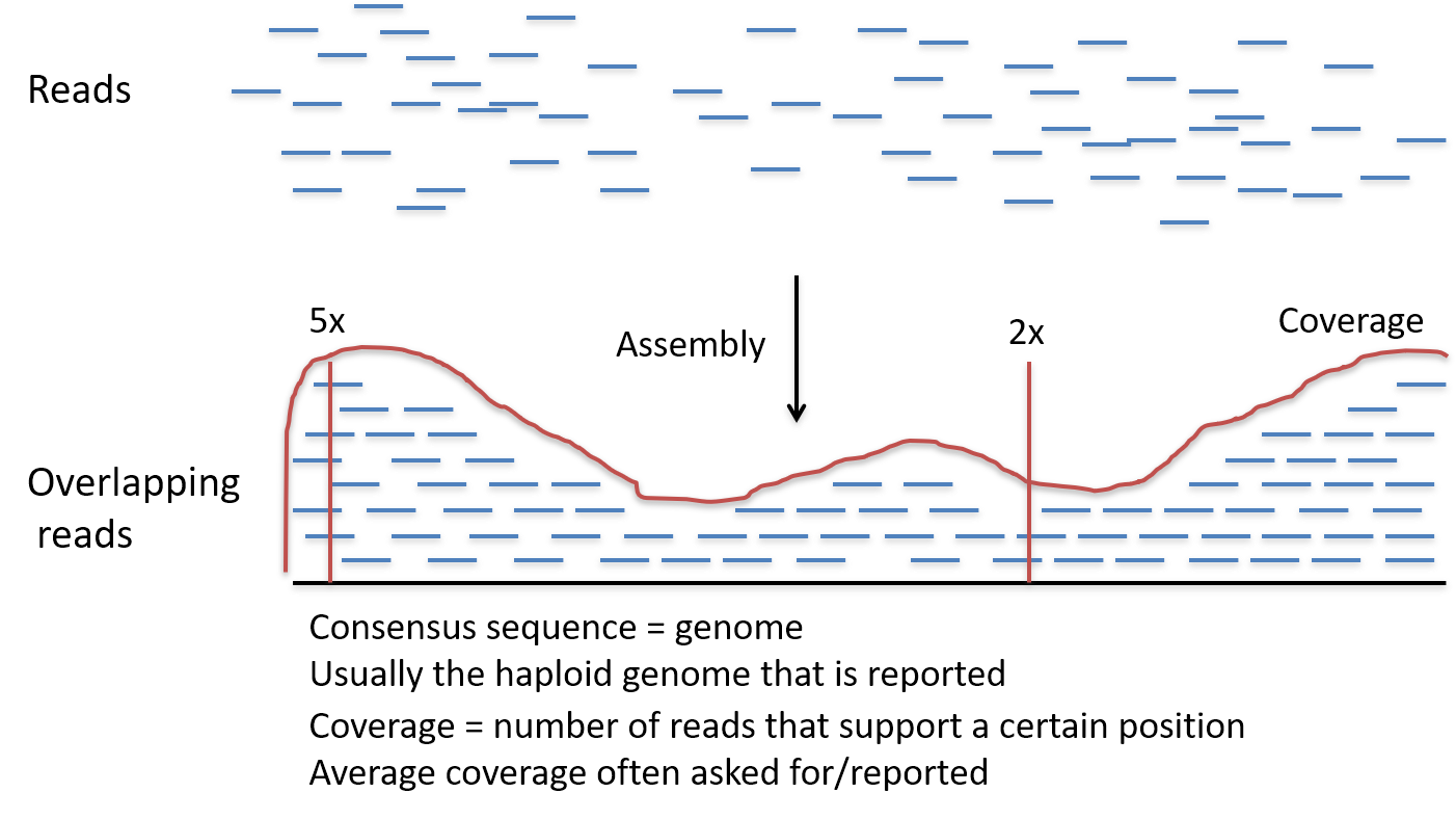
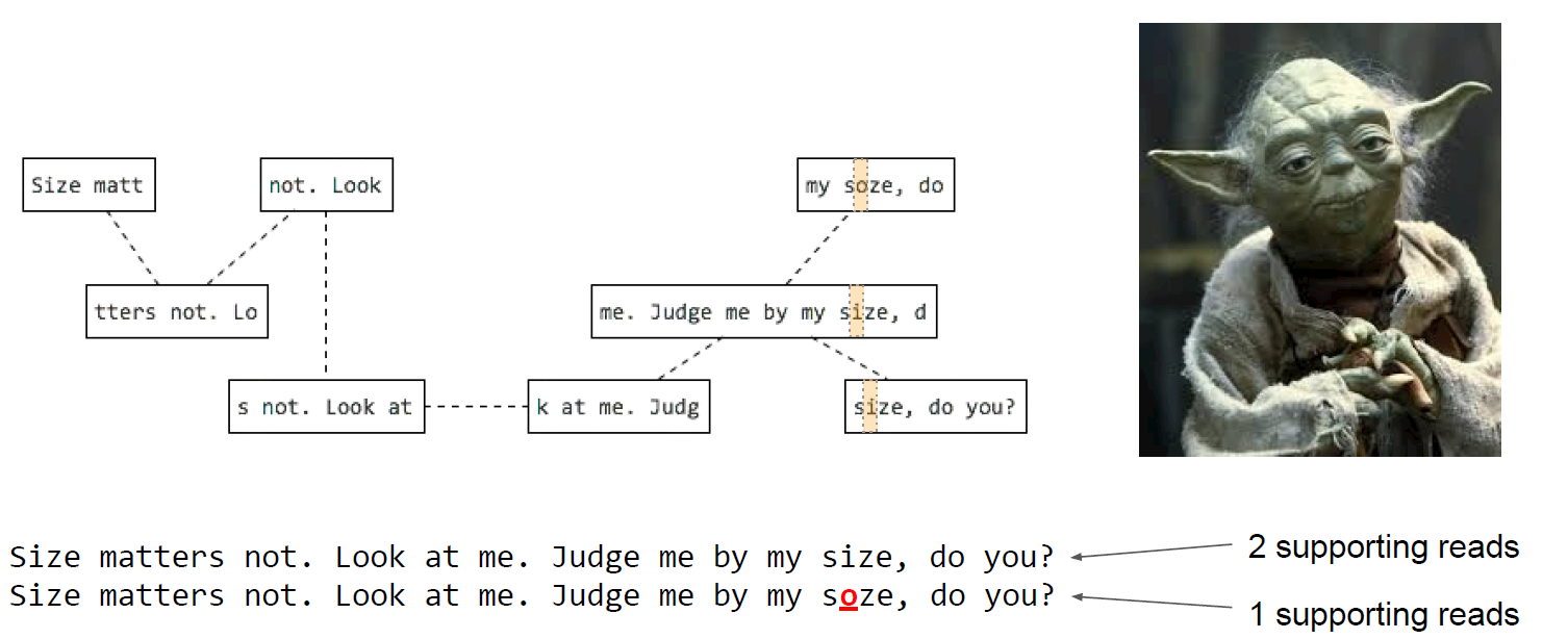
The technology of DNA sequencing? is not 100 per cent accurate and therefore there are likely to be errors in the DNA sequence that is produced.
-
So, to account for the errors that could potentially occur, each base in the genome? is sequenced a number of times over, this is called coverage. For example, 30 times (30-fold) coverage means each base? is sequenced 30 times.
-
Effectively, the more times you sequence, or
read, the same section of DNA, the more confidence you have that the final sequence is correct. 30- to 50-fold coverage is currently the standard used when sequencing human genomes to a high level of accuracy. -
During the Human Genome Project? coverage was only between 5- and 10-fold and used a different sequencing technology to those used today.
-
Coverage has increased because of a few reasons: Although most current sequencing techniques are now faster than they were during the Human Genome Project, some sequencing technologies have a higher error rate. Some sequencing technologies deal with shorter reads of DNA which means that gaps are more likely to occur when the genome is assembled. Having a higher coverage reduces the likelihood of there being gaps in the final assembled sequence. It is also much cheaper to carry out sequencing to a higher coverage than it was at the time of the Human Genome Project.
-
High coverage means that after sequencing DNA we have lots and lots of pieces of DNA sequence (reads).
-
To put this into perspective, once a human genome has been fully sequenced we have around 100 gigabases (100,000,000,000 bases) of sequence data.
-
Like the pieces of a jigsaw puzzle, these DNA reads are jumbled up so we need to piece them together and put them in the correct order to assemble the genome sequence.
Coverage calculation
Example: I know that the genome size. I am sequencing 10 Mbases genome species. I want a 50x coverage to do a good assembly. I am ordering 125 bp Illumina reads. How many reads do I need?
- (125xN)/10e+6=50
- N=(50x10e+6)/125=4e+6 (4 million reads)
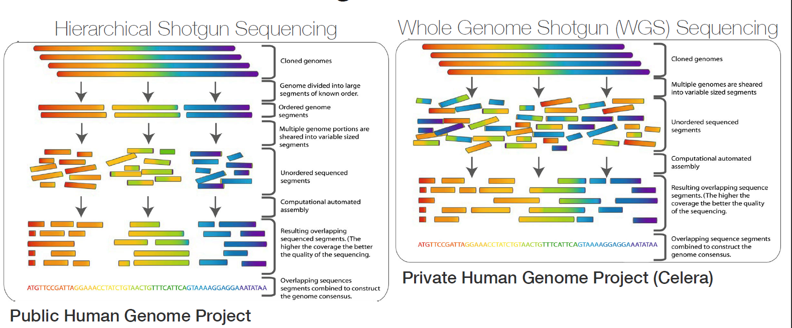
De novo assembly
-
De novo sequencing is when the genome of an organism is sequenced for the first time.
- In de novo assembly there is no existing reference genome sequence for that species to use as a template for the assembly of its genome sequence.
- If you know that the new species? is very similar to another species that does have a reference genome, it is possible to assemble the sequence using a similar genome as a guide.
- To help assemble a de novo sequence a physical gene? map can be developed before sequencing to highlight the landmarks so the scientists know where sections of DNA are located in relation to each other.
- Producing a gene map can be an expensive process, so some assembly programmes rely on data consisting of a mix of single and paired-end reads
-
Single reads are where one end or the whole of a fragment of DNA is sequenced. These sequences can then be joined together by finding overlapping regions in the sequence to create the full DNA sequence.
-
Paired-end reads are where both ends of a fragment of DNA are sequenced. The distance between paired-end reads can be anywhere between 200 base pairs? and several thousand. The key advantage of paired-end reads is that scientists know how far apart the two ends are. This makes it easier to assemble them into a continuous DNA sequence. Paired-end reads are particularly useful when assembling a de novo sequence as they provide long-range information that you wouldn’t otherwise have in the absence of a gene map.
- Assembly of a de novo sequence begins with a large number of short sections or “reads” of DNA.
- These reads are compared to each other and those sharing the same DNA sequence are grouped together.
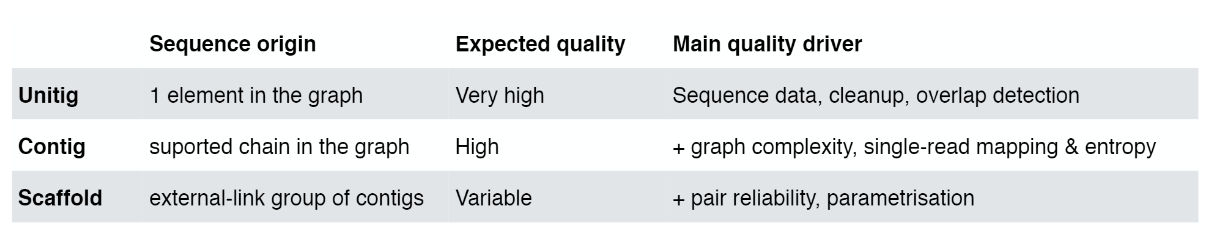
- From here they are assembled into progressively larger sections to form long contiguous (together in sequence) sequences called “contigs”.
- These contigs can then be grouped together with information taken from other technologies to provide clues for how to stitch the contigs together and roughly how far apart to place them, even if the sequence in between is still unknown. This is called “scaffolding”.
- The assembly can be further refined by ordering the individual scaffolds into chromosomes?. A physical gene map is a useful tool for doing this.
- The resulting assembly is then fed on to the next stage of the process – annotation, which identifies where the genes and other features in the sequence start and stop.
- The assembly of a genome is a computer-intensive job. It usually takes around 20 hours per gigabase of sequence for genome assembly programmes to stitch together an organism’s genome sequence from the reads of DNA sequence generated by the sequencing machines.
- So, with the 100 gigabases of sequence data we have after sequencing a human genome, it will take 2,000 hours or around 83 days to assemble the complete sequence.
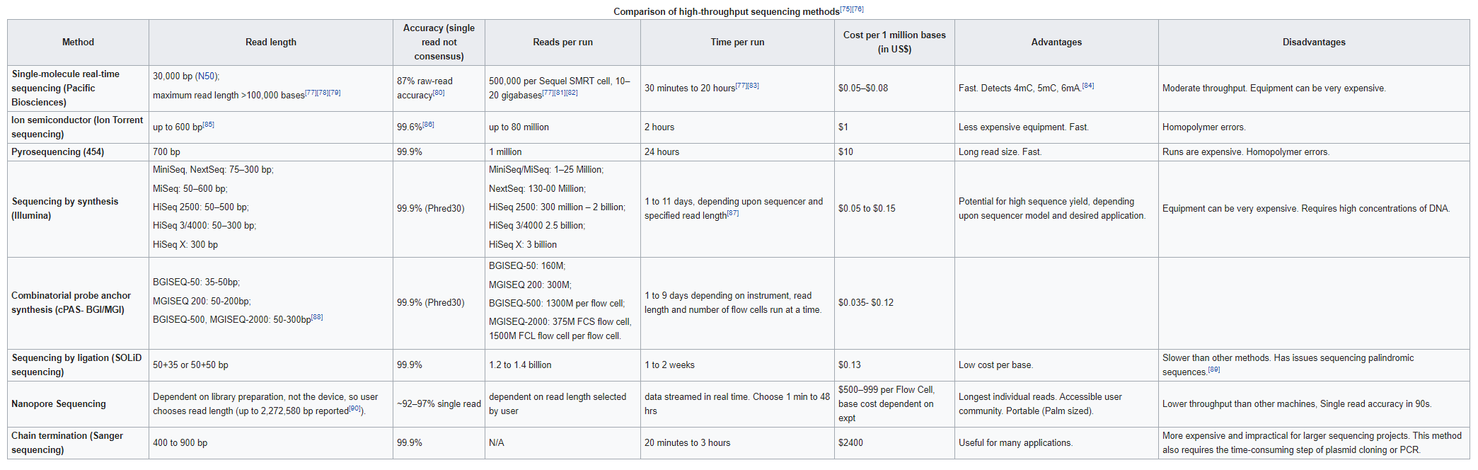
Genome assembly refers to the process of taking a large number of short DNA sequences and putting them back together to create a representation of the original chromosomes from which the DNA originated. De novo genome assemblies assume no prior knowledge of the source DNA sequence length, layout or composition. In a genome sequencing project, the DNA of the target organism is broken up into millions of small pieces and read on a sequencing machine. These “reads” vary from 20 to 1000 nucleotide base pairs (bp) in length depending on the sequencing method used. Typically for Illumina type short read sequencing, reads of length 36 - 150 bp are produced. These reads can be either single ended as described above or paired end. A good summary of other types of DNA sequencing can be found below.
Paired end reads are produced when the fragment size used in the sequencing process is much longer (typically 250 - 500 bp long) and the ends of the fragment are read in towards the middle. This produces two “paired” reads. One from the left hand end of a fragment and one from the right with a known separation distance between them. (The known separation distance is actually a distribution with a mean and standard deviation as not all original fragments are of the same length.) This extra information contained in the paired end reads can be useful for helping to tie pieces of sequence together during the assembly process.
The goal of a sequence assembler is to produce long contiguous pieces of sequence (contigs) from these reads. The contigs are sometimes then ordered and oriented in relation to one another to form scaffolds. The distances between pairs of a set of paired end reads is useful information for this purpose.
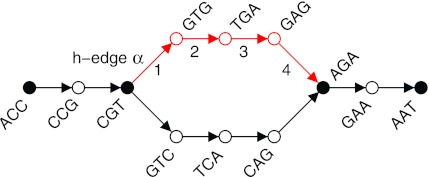
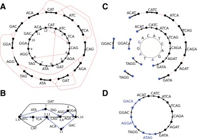
The mechanisms used by assembly software are varied but the most common type for short reads is assembly by de Bruijn graph. See this document for an explanation of the de Bruijn graph genome assembler “SPAdes.”
Genome assembly is a very difficult computational problem, made more difficult because many genomes contain large numbers of identical sequences, known as repeats. These repeats can be thousands of nucleotides long, and some occur in thousands of different locations, especially in the large genomes of plants and animals.
Why do we want to assemble an organism’s DNA?
Determining the DNA sequence of an organism is useful in fundamental research into why and how they live, as well as in applied subjects. Because of the importance of DNA to living things, knowledge of a DNA sequence may be useful in practically any biological research. For example, in medicine it can be used to identify, diagnose and potentially develop treatments for genetic diseases. Similarly, research into pathogens may lead to treatments for contagious diseases.
What do we need to do?
- Put the pieces together in the correct order to construct the complete genome sequence and identify any areas of interest.
-
This is done using processes called alignment and assembly:
Alignment is when the new DNA sequence is compared to existing DNA sequences to find any similarities or discrepancies between them and then arranged to show these features. Alignment is a vital part of assembly.Assembly involves taking a large number of DNA reads, looking for areas in which they overlap with each other and then gradually piecing together the ‘jigsaw’. It is an attempt to reconstruct the original genome. This is primarily carried out for de novo sequences?.
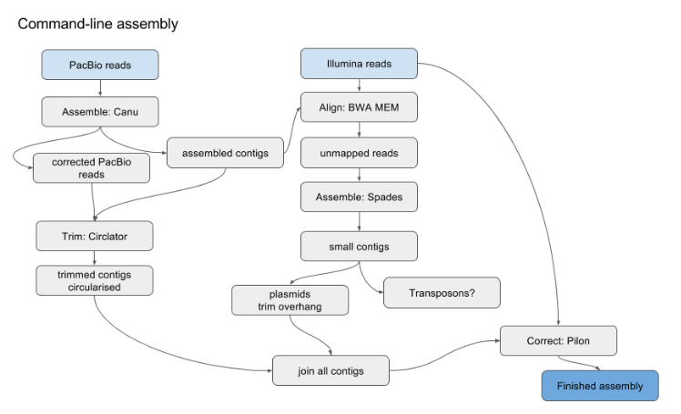
The protocol in a nutshell:
- Obtain sequence read file(s) from sequencing machine(s).
- Look at the reads - get an understanding of what you’ve got and what the quality is like.
- Raw data cleanup/quality trimming if necessary.
- Choose an appropriate assembly parameter set.
- Assemble the data into contigs/scaffolds.
- Examine the output of the assembly and assess assembly quality.
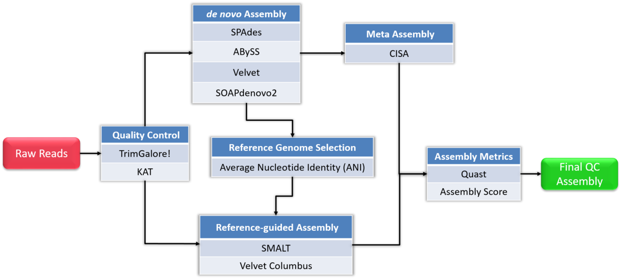
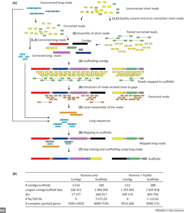
Flowchart of de novo assembly protocol.
Long read sequencing
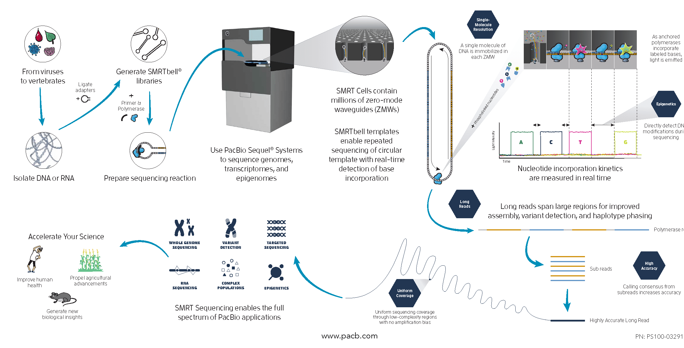
Single Molecule, Real-Time (SMRT) Sequencing is the core technology powering our long-read sequencing platforms. This innovative approach was the first of its kind and is now a proven technology used in all fields of life science.
Long Reads (PacBio)
With reads tens of kilobases in length you can readily assemble complete genomes and sequence full-length transcripts.
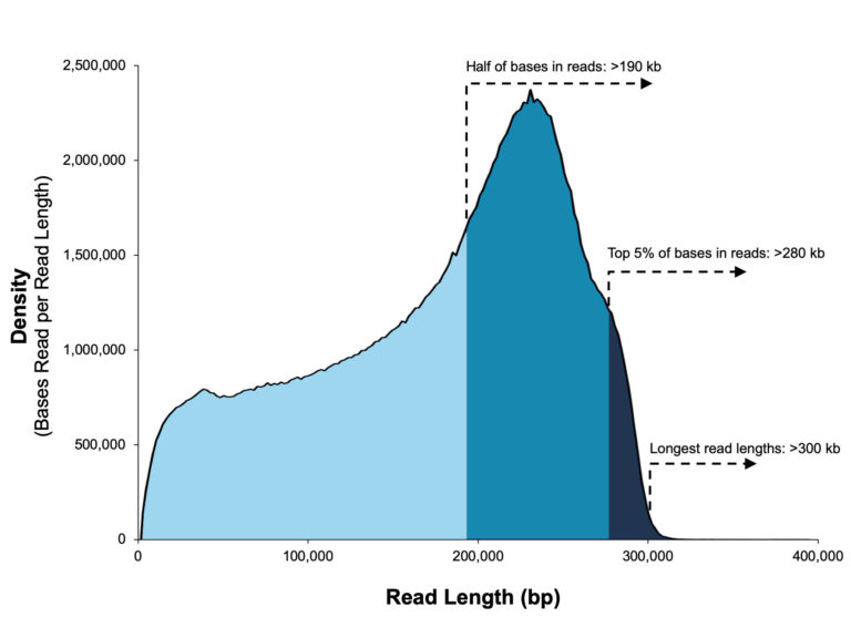 A 20 kb size-selected human library using the SMRTbell Express Template Prep Kit 2.0 on a Sequel II System (2.0 Chemistry, Sequel II System Software v8.0, 30-hour movie).
SMRT Sequencing enables simultaneous collection of data from millions of wells using the natural process of DNA replication to sequence long fragments of native DNA or RNA.
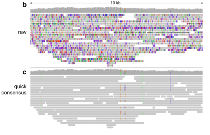
PacBio Error
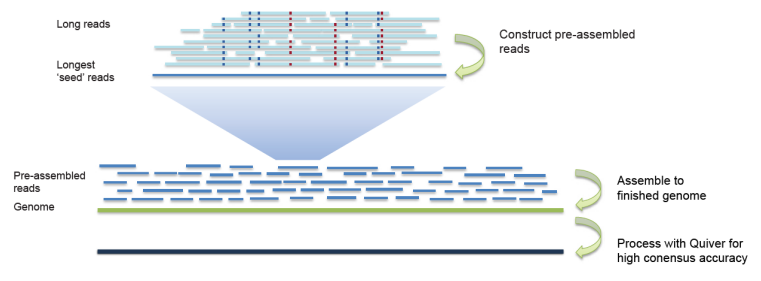
Long Reads Assembly
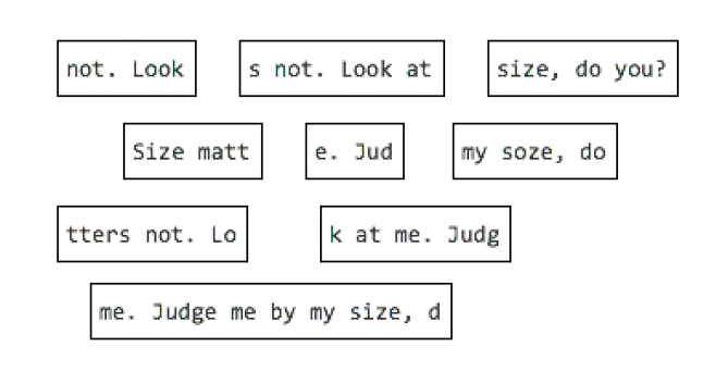
OLC Algorithm
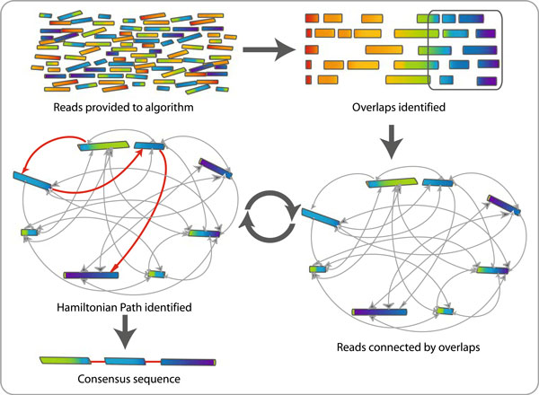
OLC example
Long reads publications
- Mitsuhashi, Satomi et al. (2019) Long-read sequencing for rare human genetic diseases. Journal of human genetics
- Wenger, Aaron M et al. (2019) Accurate circular consensus long-read sequencing improves variant detection and assembly of a human genome. Nature biotechnology
- Eichler, Evan E et al. (2019) Genetic Variation, Comparative Genomics, and the Diagnosis of Disease. The New England journal of medicine
- Mantere, Tuomo et al. (2019) Long-Read Sequencing Emerging in Medical Genetics Frontiers in genetics
- Wang, Bo et al. (2019) Reviving the Transcriptome Studies: An Insight into the Emergence of Single-molecule Transcriptome Sequencing Frontiers in genetics
- Pollard, Martin O et al. (2018) Long reads: their purpose and place. Human molecular genetics
- Sedlazeck, Fritz J et al. (2018) Accurate detection of complex structural variations using single-molecule sequencing. Nature methods
- Ardui, Simon et al. (2018) Single molecule real-time (SMRT) sequencing comes of age: applications and utilities for medical diagnostics. Nucleic acids research
- Nakano, Kazuma et al. (2017) Advantages of genome sequencing by long-read sequencer using SMRT technology in medical area. Human cell
- Chaisson, Mark J P et al. (2015) Genetic variation and the de novo assembly of human genomes. Nature reviews. Genetics
- Rhoads, Anthony et al. (2015) PacBio sequencing and its applications. Genomics, proteomics & bioinformatics
- Berlin, Konstantin et al. (2015) Assembling large genomes with single-molecule sequencing and locality-sensitive hashing. Nature biotechnology
- Huddleston, John et al. (2014) Reconstructing complex regions of genomes using long-read sequencing technology. Genome research
- Koren, Sergey et al. (2013) Reducing assembly complexity of microbial genomes with single-molecule sequencing. Genome biology
- Travers, Kevin J et al. (2010) A flexible and efficient template format for circular consensus sequencing and SNP detection. Nucleic acids research
- Flusberg, Benjamin A et al. (2010) Direct detection of DNA methylation during single-molecule, real-time sequencing. Nature methods
- Eid, John et al. (2009) Real-time DNA sequencing from single polymerase molecules. Science
Repeat in Genome
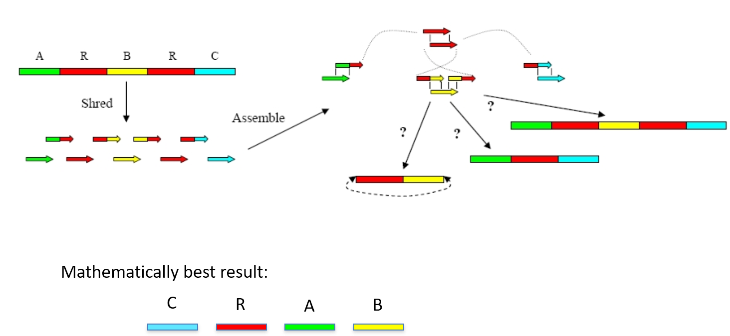
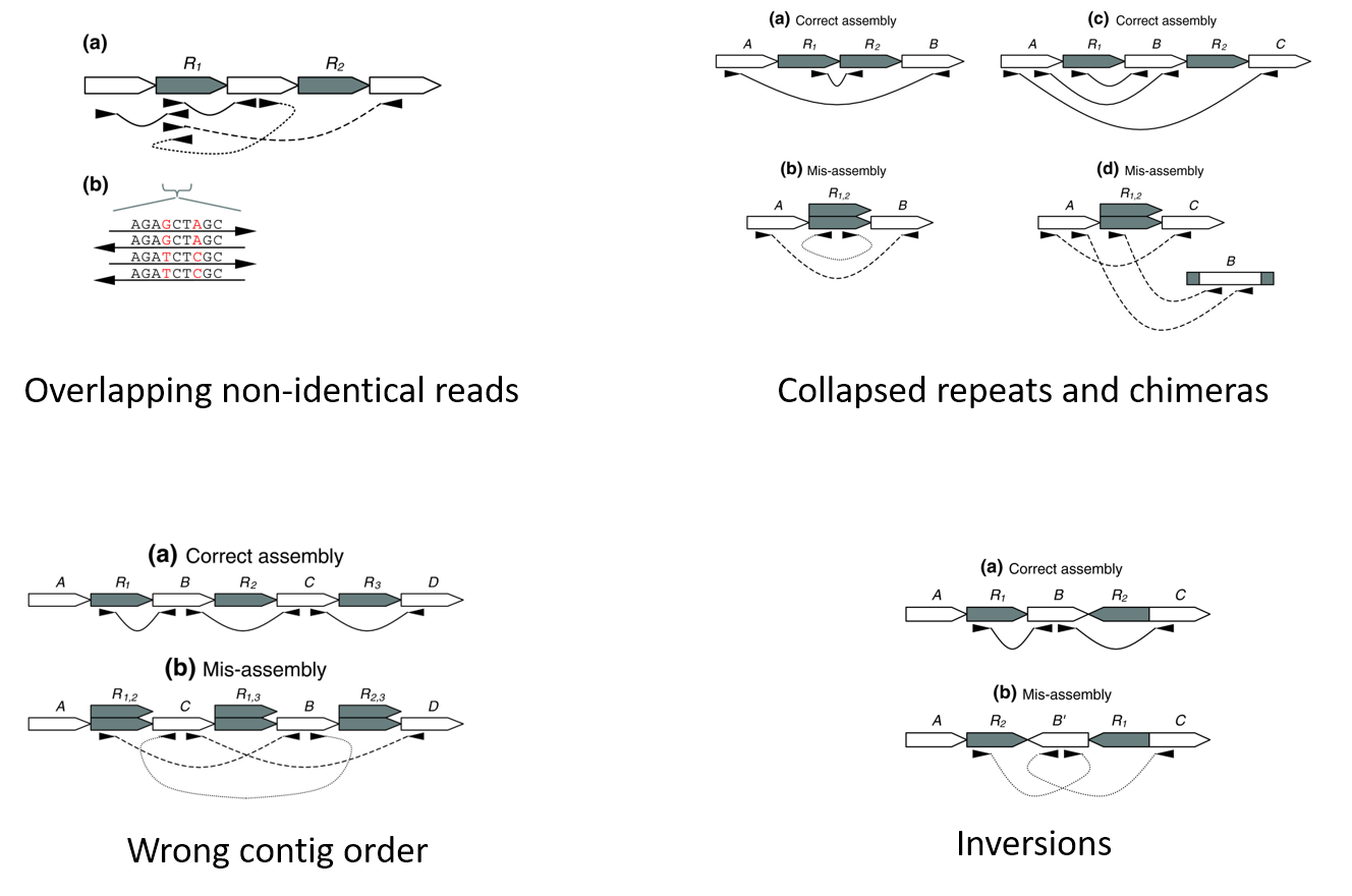
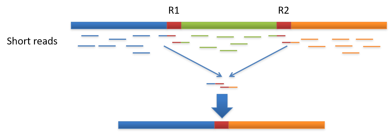

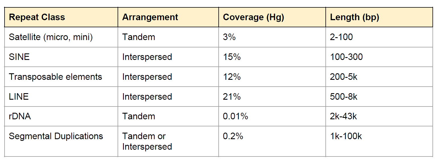
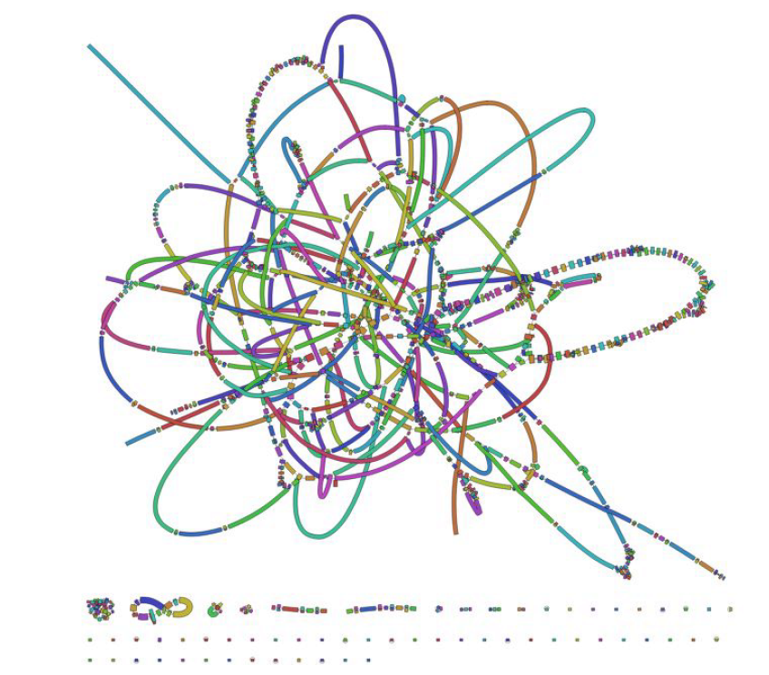 Fig: E.coli genome (4.6Mbp)
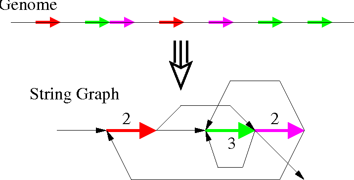
String Graph Algorithm
Hybrid Assembly
Genome assembly complexity
GC-content
- Regions of low or high GC-content have a lower coverage (Illumina, not PacBio)
Secondary structure
- Regions that are tightly bound get less coverage
Ploidy level
- On higher ploidy levels you potentially have more alleles present
Size of organism
- Hard to extract enough DNA from small organisms
Pooled individuals
- Increases the variability of the DNA (more alleles)
Inhibiting compounds
- Lower coverage and shorter fragments
Presence of additional genomes/contamination
- Lower coverage of what you actually are interested in, potentially chimeric assemblies
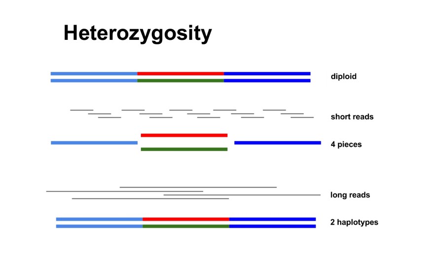
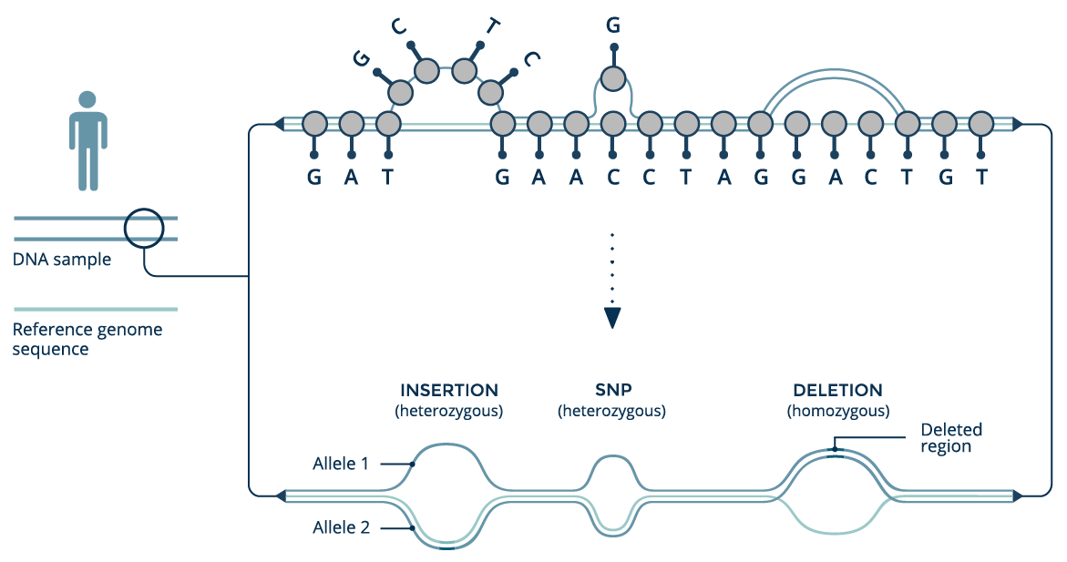
Heterozygosity
Haplotype
Contiguity
- Fewer contigs
- Longer contigs
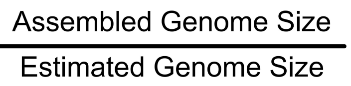
Completeness : Total size
Proportion of the original genome represented by the assembly Can be between 0 and 1
Completeness: core genes
-
Proportion of coding sequences can be estimated based on known core genes thought to be present in a wide variety of organisms.
-
Assumes that the proportion of assembled genes is equal to the proportion of assembled core genes.
Correctness
Proportion of the assembly that is free from errors
Errors include
- Mis-joins
- Repeat compressions
- Unnecessary duplications
- Indels / SNPs caused by assembler
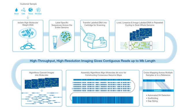
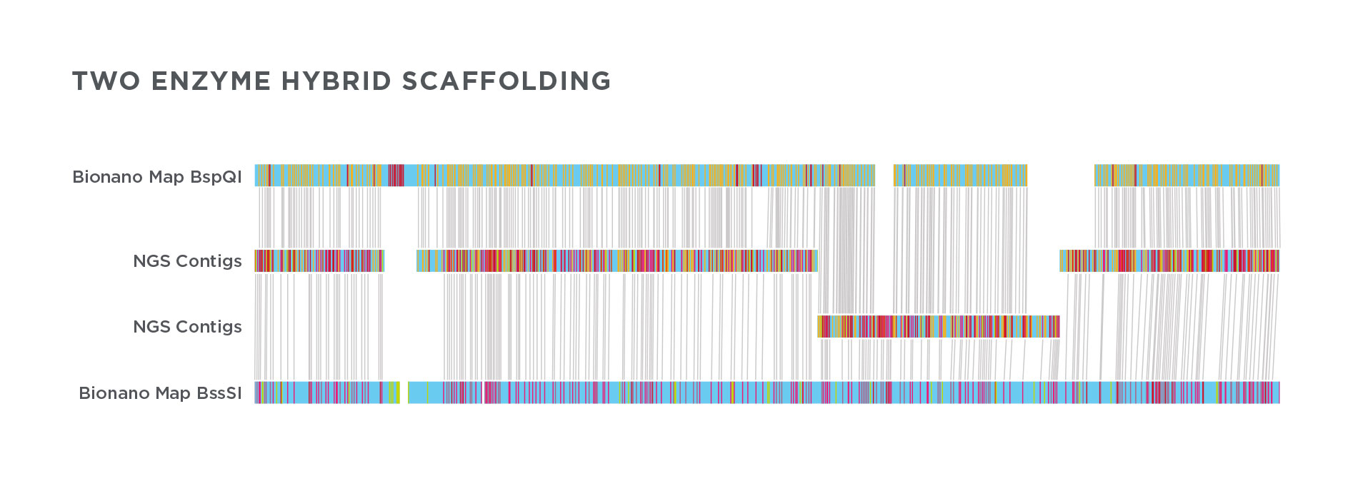
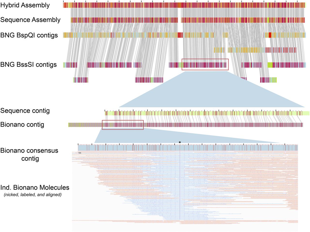
Optical mapping
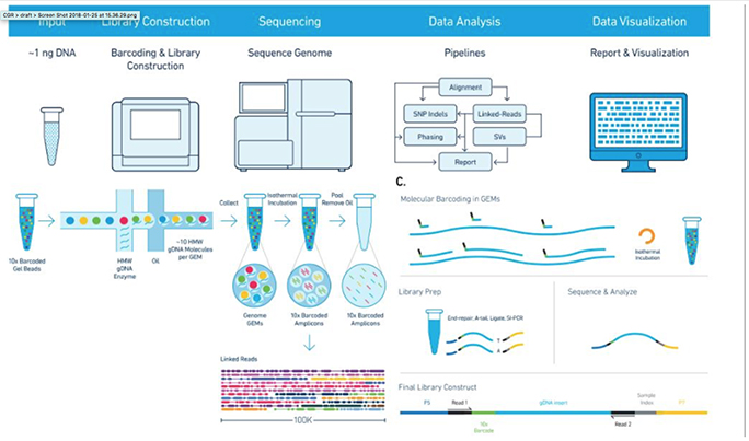
10x Genomics
Assembly results
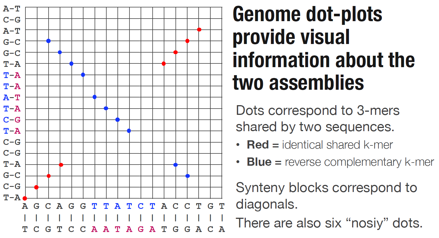
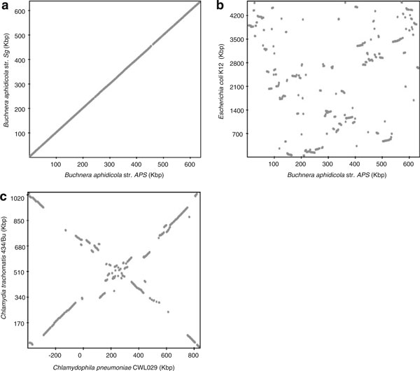
Dotplot
Metrics
- Number of contigs
- Average contig length
- Median contig length
- Maximum contig length
- “N50”, “NG50”, “D50”
N50

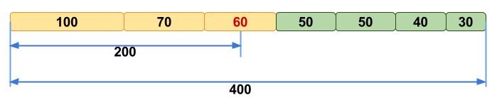
N50 example
| Contig Length | Cumulative Sum |
|---|---|
| 100 | 100 |
| 200 | 300 |
| 230 | 530 |
| 400 | 930 |
| 750 | 1680 |
| 852 | 2532 |
| 950 | 3482 |
| 990 | 4472 |
| 1020 | 5492 |
| 1278 | 6770 |
| 1280 | 8050 |
| 1290 | 9340 |
Check Genome Size by Illumina Reads
cd /data/gpfs/assoc/bch709-1/<YOUR_ID>/
mkdir -p Genome_assembly/Illumina
cd Genome_assembly/Illumina
Create Preprocessing Env
conda create -n preprocessing python=3 -y

conda activate preprocessing

conda install -c bioconda trim-galore jellyfish=2.2.10 'multiqc<1.34' nanostat nanoplot -y
Reads Download
https://www.dropbox.com/s/ax38m9wra44lsgi/WGS_R1.fq.gz
https://www.dropbox.com/s/kp7et2du5c2v385/WGS_R2.fq.gz
Count Reads Number in file
echo $(zcat WGS_R1.fq.gz |wc -l)/4 | bc

echo $(cat WGS_R1.fq |wc -l)/4 | bc
Advanced approach
for i in `ls -1 *.fq.gz`; do echo $(zcat ${i} | wc -l)/4|bc; done


***For all gzip compressed fastq files, display the number of reads since 4 lines = 1 reads***
Reads Trimming
#!/bin/bash
#SBATCH --job-name=Trim
#SBATCH --cpus-per-task=8
#SBATCH --time=2:00:00
#SBATCH --mem=30g
#SBATCH --account=cpu-s2-bch709-1
#SBATCH --partition=cpu-s2-core-0
#SBATCH --mail-type=all
#SBATCH --mail-user=<YOUR ID>@unr.edu

trim_galore --paired   --three_prime_clip_R1 10 --three_prime_clip_R2 10 --cores 8  --max_n 40  -o trimmed_fastq --fastqc <READ_R1> <READ_R2>

multiqc . -n WGS_Illumina --exclude rsem --exclude gatk
Why assemble genomes
- Produce a reference for new species
- Genomic variation can be studied by comparing against the reference
- A wide variety of molecular biological tools become available or more effective
- Coding sequences can be studied in the context of their related non-coding (eg regulatory) sequences
- High level genome structure (number, arrangement of genes and repeats) can be studied
Assembly is very challenging (“impossible”) because
- Sequencing bias under represents certain regions
- Reads are short relative to genome size
- Repeats create tangled hubs in the assembly graph
- Sequencing errors cause detours and bubbles in the assembly graph
Prerequisite
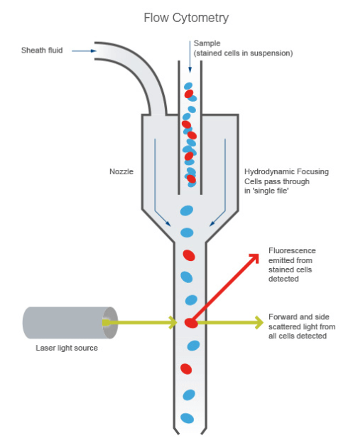
Flow Cytometry
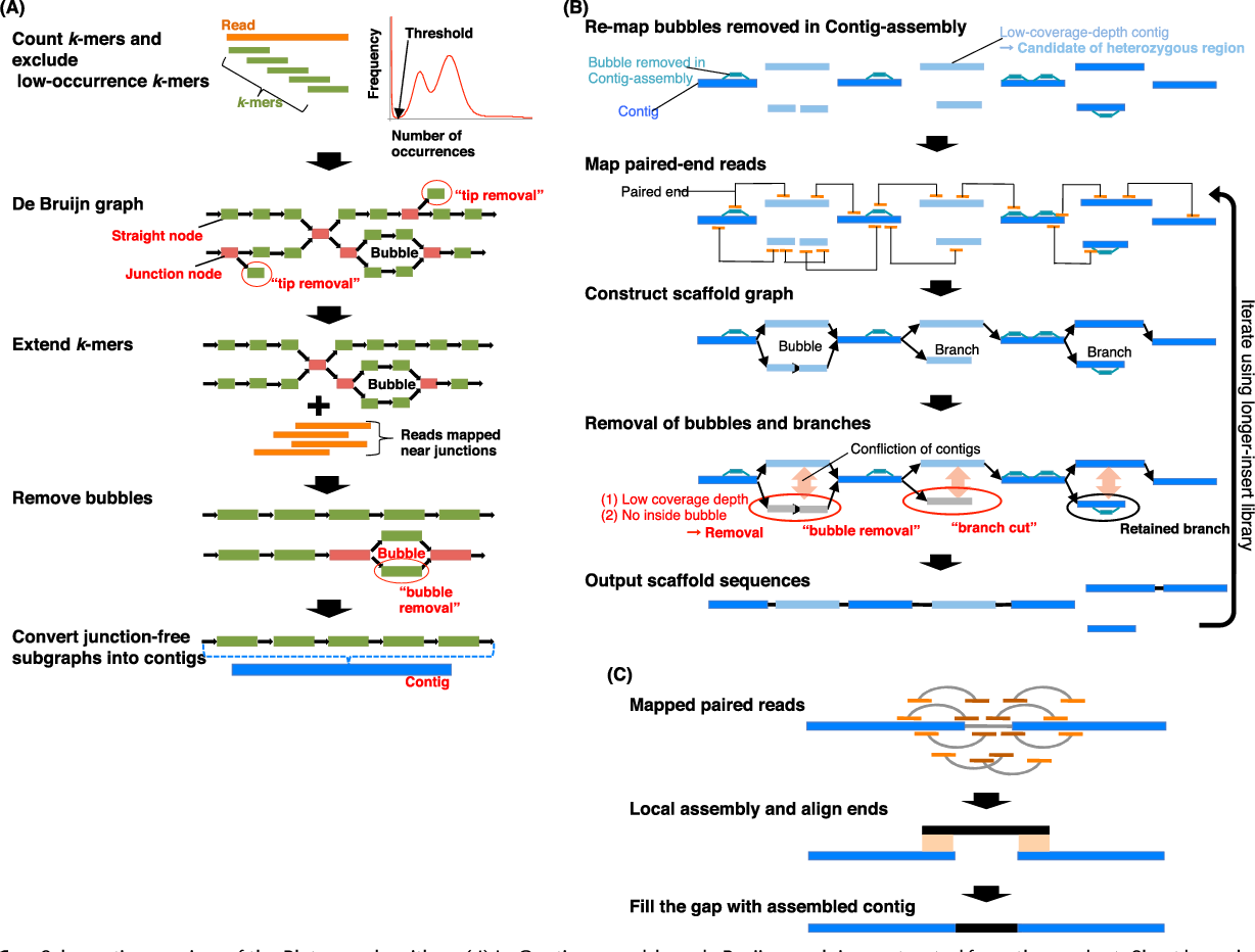
K-mer spectrum
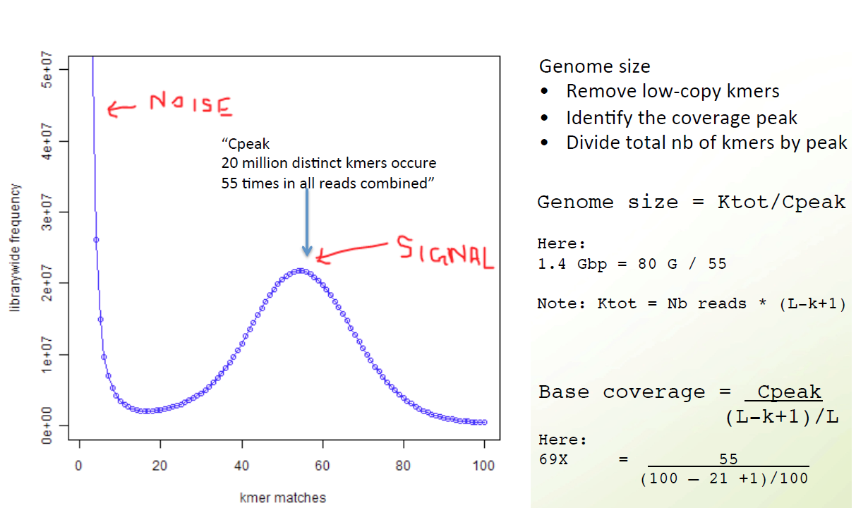
K-mer counting
mkdir kmer && cd kmer
#!/bin/bash
#SBATCH --job-name=Trim
#SBATCH --cpus-per-task=10
#SBATCH --time=2:00:00
#SBATCH --mem=10g
#SBATCH --account=cpu-s2-bch709-1
#SBATCH --partition=cpu-s2-core-0
#SBATCH --mail-type=all
#SBATCH --mail-user=<YOUR ID>@unr.edu
#SBATCH -o trim.out # STDOUT
#SBATCH -e trim.err # STDERR
gunzip ../trimmed_fastq/*.gz
jellyfish count -C -m 21 -s 100000000 -t 10 ../trimmed_fastq/*.fq -o reads.jf
jellyfish histo -t 10 reads.jf > reads_jf.histo
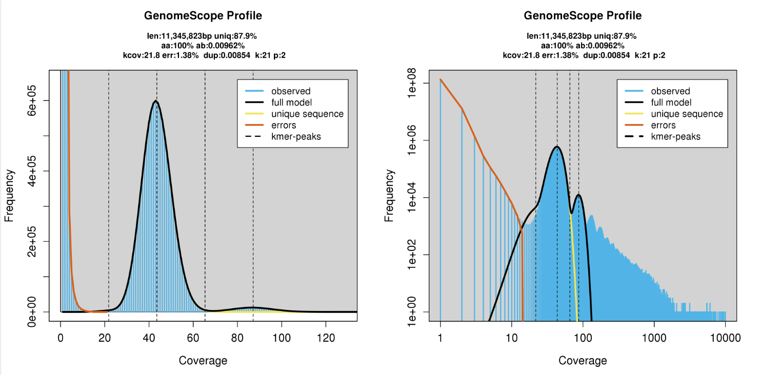
Upload to GenomeScope
http://qb.cshl.edu/genomescope/genomescope2.0
Genome assembly Spades
cd /data/gpfs/assoc/bch709-1/<YOURID>/Genome_assembly/Illumina/
mkdir Spades
cd Spades
conda create -n genomeassembly -y
conda activate genomeassembly
conda install -c bioconda spades canu pacbio_falcon samtools minimap2 'multiqc<1.34'  openssl=1.0 -y
conda install -c r r-ggplot2 r-stringr r-scales r-argparse -y
#!/bin/bash
#SBATCH --job-name=Spades
#SBATCH --cpus-per-task=32
#SBATCH --time=2:00:00
#SBATCH --mem=64g
#SBATCH --account=cpu-s2-bch709-1
#SBATCH --partition=cpu-s2-core-0
#SBATCH --mail-type=all
#SBATCH --mail-user=<YOUR ID>@unr.edu
#SBATCH -o Spades.out # STDOUT
#SBATCH -e Spades.err # STDERR

spades.py -k 21,33,55,77 --careful -1 <trim_galore output> -2 <trim_galore output> -o spades_output --memory 64 --threads 32
###Spade
Log
Command line: /data/gpfs/home/wyim/miniconda3/envs/genomeassembly/bin/spades.py -k21,33,55,77     --careful       -1      /data/gpfs/assoc/bch709-1/wyim/gee/trimmed_fastq/WGS_R1_val_1.fq.gz    -2      /data/gpfs/assoc/bch709-1/wyim/gee/trimmed_fastq/WGS_R2_val_2.fq.gz    -o      /data/gpfs/assoc/bch709-1/wyim/gee/spades_output       --memory        120     --threads       32

System information:
  SPAdes version: 3.13.1
  Python version: 3.7.3
  OS: Linux-3.10.0-957.27.2.el7.x86_64-x86_64-with-centos-7.6.1810-Core

Output dir: /data/gpfs/assoc/bch709-1/wyim/gee/spades_output
Mode: read error correction and assembling
Debug mode is turned OFF

Dataset parameters:
  Multi-cell mode (you should set '--sc' flag if input data was obtained with MDA (single-cell) technology or --meta flag if processing metagenomic dataset)
  Reads:
    Library number: 1, library type: paired-end
      orientation: fr
      left reads: ['/data/gpfs/assoc/bch709-1/wyim/gee/trimmed_fastq/WGS_R1_val_1.fq.gz']
      right reads: ['/data/gpfs/assoc/bch709-1/wyim/gee/trimmed_fastq/WGS_R2_val_2.fq.gz']
      interlaced reads: not specified
      single reads: not specified
      merged reads: not specified
Read error correction parameters:
  Iterations: 1
  PHRED offset will be auto-detected
  Corrected reads will be compressed
Assembly parameters:
  k: [21, 33, 55, 77]
  Repeat resolution is enabled
  Mismatch careful mode is turned ON
  MismatchCorrector will be used
  Coverage cutoff is turned OFF
Other parameters:
  Dir for temp files: /data/gpfs/assoc/bch709-1/wyim/gee/spades_output/tmp
  Threads: 64
  Memory limit (in Gb): 140


======= SPAdes pipeline started. Log can be found here: /data/gpfs/assoc/bch709-1/wyim/gee/spades_output/spades.log


===== Read error correction started.


== Running read error correction tool: /data/gpfs/home/wyim/miniconda3/envs/genomeassembly/bin/spades-hammer /data/gpfs/assoc/bch709-1/wyim/gee/spades_output/corrected/configs/config.info

  0:00:00.000     4M / 4M    INFO    General                 (main.cpp                  :  75)   Starting BayesHammer, built from N/A, git revision N/A
  0:00:00.000     4M / 4M    INFO    General                 (main.cpp                  :  76)   Loading config from /data/gpfs/assoc/bch709-1/wyim/gee/spades_output/corrected/configs/config.info
  0:00:00.001     4M / 4M    INFO    General                 (main.cpp                  :  78)   Maximum # of threads to use (adjusted due to OMP capabilities): 32
  0:00:00.001     4M / 4M    INFO    General                 (memory_limit.cpp          :  49)   Memory limit set to 140 Gb
  0:00:00.001     4M / 4M    INFO    General                 (main.cpp                  :  86)   Trying to determine PHRED offset
  0:00:00.038     4M / 4M    INFO    General                 (main.cpp                  :  92)   Determined value is 33
  0:00:00.038     4M / 4M    INFO    General                 (hammer_tools.cpp          :  36)   Hamming graph threshold tau=1, k=21, subkmer positions = [ 0 10 ]
  0:00:00.038     4M / 4M    INFO    General                 (main.cpp                  : 113)   Size of aux. kmer data 24 bytes
     === ITERATION 0 begins ===
  0:00:00.042     4M / 4M    INFO   K-mer Index Building     (kmer_index_builder.hpp    : 301)   Building kmer index
  0:00:00.042     4M / 4M    INFO    General                 (kmer_index_builder.hpp    : 117)   Splitting kmer instances into 512 files using 32 threads. This might take a while.
  0:00:00.043     4M / 4M    INFO    General                 (file_limit.hpp            :  32)   Open file limit set to 65536
  0:00:00.043     4M / 4M    INFO    General                 (kmer_splitters.hpp        :  89)   Memory available for splitting buffers: 1.45829 Gb
  0:00:00.043     4M / 4M    INFO    General                 (kmer_splitters.hpp        :  97)   Using cell size of 131072
  0:00:02.300    17G / 17G   INFO   K-mer Splitting          (kmer_data.cpp             :  97)   Processing /data/gpfs/assoc/bch709-1/wyim/gee/trimmed_fastq/WGS_R1_val_1.fq.gz
  0:00:19.373    17G / 18G   INFO   K-mer Splitting          (kmer_data.cpp             : 107)   Processed 3022711 reads
  0:00:19.373    17G / 18G   INFO   K-mer Splitting          (kmer_data.cpp             :  97)   Processing /data/gpfs/assoc/bch709-1/wyim/gee/trimmed_fastq/WGS_R2_val_2.fq.gz
  0:00:37.483    17G / 18G   INFO   K-mer Splitting          (kmer_data.cpp             : 107)   Processed 6045422 reads
  0:00:37.483    17G / 18G   INFO   K-mer Splitting          (kmer_data.cpp             : 112)   Total 6045422 reads processed
  0:00:39.173   128M / 18G   INFO    General                 (kmer_index_builder.hpp    : 120)   Starting k-mer counting.
  0:00:43.628   128M / 18G   INFO    General                 (kmer_index_builder.hpp    : 127)   K-mer counting done. There are 318799406 kmers in total.
  0:00:43.628   128M / 18G   INFO    General                 (kmer_index_builder.hpp    : 133)   Merging temporary buckets.
  0:00:48.548   128M / 18G   INFO   K-mer Index Building     (kmer_index_builder.hpp    : 314)   Building perfect hash indices
  0:00:58.437   320M / 18G   INFO    General                 (kmer_index_builder.hpp    : 150)   Merging final buckets.
  0:01:00.516   320M / 18G   INFO   K-mer Index Building     (kmer_index_builder.hpp    : 336)   Index built. Total 147835808 bytes occupied (3.70981 bits per kmer).
  0:01:00.518   320M / 18G   INFO   K-mer Counting           (kmer_data.cpp             : 356)   Arranging kmers in hash map order
  0:02:50.247     5G / 18G   INFO    General                 (main.cpp                  : 148)   Clustering Hamming graph.
  0:05:15.609     5G / 18G   INFO    General                 (main.cpp                  : 155)   Extracting clusters
  0:06:20.894     5G / 18G   INFO    General                 (main.cpp                  : 167)   Clustering done. Total clusters: 47999941
  0:06:20.900     2G / 18G   INFO   K-mer Counting           (kmer_data.cpp             : 376)   Collecting K-mer information, this takes a while.
  0:06:23.367     9G / 18G   INFO   K-mer Counting           (kmer_data.cpp             : 382)   Processing /data/gpfs/assoc/bch709-1/wyim/gee/trimmed_fastq/WGS_R1_val_1.fq.gz
  0:06:41.328     9G / 18G   INFO   K-mer Counting           (kmer_data.cpp             : 382)   Processing /data/gpfs/assoc/bch709-1/wyim/gee/trimmed_fastq/WGS_R2_val_2.fq.gz
  0:06:59.453     9G / 18G   INFO   K-mer Counting           (kmer_data.cpp             : 389)   Collection done, postprocessing.
  0:07:00.669     9G / 18G   INFO   K-mer Counting           (kmer_data.cpp             : 403)   There are 318799406 kmers in total. Among them 268145204 (84.1109%) are singletons.
  0:07:00.669     9G / 18G   INFO    General                 (main.cpp                  : 173)   Subclustering Hamming graph
  0:15:33.177     9G / 18G   INFO   Hamming Subclustering    (kmer_cluster.cpp          : 649)   Subclustering done. Total 11739 non-read kmers were generated.
  0:15:33.177     9G / 18G   INFO   Hamming Subclustering    (kmer_cluster.cpp          : 650)   Subclustering statistics:
  0:15:33.177     9G / 18G   INFO   Hamming Subclustering    (kmer_cluster.cpp          : 651)     Total singleton hamming clusters: 31640728. Among them 6970 (0.0220286%) are good
  0:15:33.177     9G / 18G   INFO   Hamming Subclustering    (kmer_cluster.cpp          : 652)     Total singleton subclusters: 14379. Among them 2710 (18.8469%) are good
  0:15:33.177     9G / 18G   INFO   Hamming Subclustering    (kmer_cluster.cpp          : 653)     Total non-singleton subcluster centers: 20505272. Among them 19729791 (96.2181%) are good
  0:15:33.177     9G / 18G   INFO   Hamming Subclustering    (kmer_cluster.cpp          : 654)     Average size of non-trivial subcluster: 14.0052 kmers
  0:15:33.177     9G / 18G   INFO   Hamming Subclustering    (kmer_cluster.cpp          : 655)     Average number of sub-clusters per non-singleton cluster: 1.25432  0:15:33.177     9G / 18G   INFO   Hamming Subclustering    (kmer_cluster.cpp          : 656)     Total solid k-mers: 19739471
  0:15:33.177     9G / 18G   INFO   Hamming Subclustering    (kmer_cluster.cpp          : 657)     Substitution probabilities: [4,4]((0.944751,0.0179573,0.0182179,0.0190737),(0.0183827,0.9447,0.0178155,0.0191018),(0.0189441,0.0177016,0.94483,0.0185242),(0.0190054,0.0181679,0.0179184,0.944908))
  0:15:33.233     9G / 18G   INFO    General                 (main.cpp                  : 178)   Finished clustering.
  0:15:33.233     9G / 18G   INFO    General                 (main.cpp                  : 197)   Starting solid k-mers expansion in 32 threads.
  0:16:01.042     9G / 18G   INFO    General                 (main.cpp                  : 218)   Solid k-mers iteration 0 produced 1807215 new k-mers.
  0:16:28.728     9G / 18G   INFO    General                 (main.cpp                  : 218)   Solid k-mers iteration 1 produced 152036 new k-mers.
  0:16:56.455     9G / 18G   INFO    General                 (main.cpp                  : 218)   Solid k-mers iteration 2 produced 13249 new k-mers.
  0:17:24.110     9G / 18G   INFO    General                 (main.cpp                  : 218)   Solid k-mers iteration 3 produced 1204 new k-mers.
  0:17:51.837     9G / 18G   INFO    General                 (main.cpp                  : 218)   Solid k-mers iteration 4 produced 93 new k-mers.
  0:18:19.634     9G / 18G   INFO    General                 (main.cpp                  : 218)   Solid k-mers iteration 5 produced 20 new k-mers.
  0:18:47.540     9G / 18G   INFO    General                 (main.cpp                  : 218)   Solid k-mers iteration 6 produced 7 new k-mers.
  0:18:47.540     9G / 18G   INFO    General                 (main.cpp                  : 222)   Solid k-mers finalized
  0:18:47.540     9G / 18G   INFO    General                 (hammer_tools.cpp          : 220)   Starting read correction in 32 threads.
  0:18:47.540     9G / 18G   INFO    General                 (hammer_tools.cpp          : 233)   Correcting pair of reads: /data/gpfs/assoc/bch709-1/wyim/gee/trimmed_fastq/WGS_R1_val_1.fq.gz and /data/gpfs/assoc/bch709-1/wyim/gee/trimmed_fastq/WGS_R2_val_2.fq.gz
  0:19:07.696    12G / 18G   INFO    General                 (hammer_tools.cpp          : 168)   Prepared batch 0 of 3022711 reads.
  0:19:28.112    12G / 18G   INFO    General                 (hammer_tools.cpp          : 175)   Processed batch 0
  0:19:33.861    12G / 18G   INFO    General                 (hammer_tools.cpp          : 185)   Written batch 0
  0:19:35.020     9G / 18G   INFO    General                 (hammer_tools.cpp          : 274)   Correction done. Changed 10322067 bases in 4896755 reads.
  0:19:35.020     9G / 18G   INFO    General                 (hammer_tools.cpp          : 275)   Failed to correct 299 bases out of 782307432.
  0:19:35.053   128M / 18G   INFO    General                 (main.cpp                  : 255)   Saving corrected dataset description to /data/gpfs/assoc/bch709-1/wyim/gee/spades_output/corrected/corrected.yaml
  0:19:35.054   128M / 18G   INFO    General                 (main.cpp                  : 262)   All done. Exiting.

== Compressing corrected reads (with pigz)

== Dataset description file was created: /data/gpfs/assoc/bch709-1/wyim/gee/spades_output/corrected/corrected.yaml


===== Read error correction finished.


===== Assembling started.


===== Mismatch correction finished.

 * Corrected reads are in /data/gpfs/assoc/bch709-1/wyim/gee/spades_output/corrected/
 * Assembled contigs are in /data/gpfs/assoc/bch709-1/wyim/gee/spades_output/contigs.fasta
 * Assembled scaffolds are in /data/gpfs/assoc/bch709-1/wyim/gee/spades_output/scaffolds.fasta
 * Paths in the assembly graph corresponding to the contigs are in /data/gpfs/assoc/bch709-1/wyim/gee/spades_output/contigs.paths
 * Paths in the assembly graph corresponding to the scaffolds are in /data/gpfs/assoc/bch709-1/wyim/gee/spades_output/scaffolds.paths
 * Assembly graph is in /data/gpfs/assoc/bch709-1/wyim/gee/spades_output/assembly_graph.fastg
 * Assembly graph in GFA format is in /data/gpfs/assoc/bch709-1/wyim/gee/spades_output/assembly_graph_with_scaffolds.gfa

======= SPAdes pipeline finished.

SPAdes log can be found here: /data/gpfs/assoc/bch709-1/wyim/gee/spades_output/spades.log

Thank you for using SPAdes!
Assembly statistics
N50 example
N50 is a measure to describe the quality of assembled genomes that are fragmented in contigs of different length. The N50 is defined as the minimum contig length needed to cover 50% of the genome.
| Contig Length |
|---|
| 100 |
| 200 |
| 230 |
| 400 |
| 750 |
| 852 |
| 950 |
| 990 |
| 1020 |
| 1278 |
| 1280 |
| 1290 |
conda install -c bioconda -c conda-forge assembly-stats
cd spades_output
assembly-stats scaffolds.fasta
assembly-stats contigs.fasta
Assembly statistics result
stats for scaffolds.fasta
sum = 11241648, n = 2345, ave = 4793.88, largest = 677246
N50 = 167555, n = 17
N60 = 124056, n = 24
N70 = 97565, n = 34
N80 = 72177, n = 48
N90 = 38001, n = 68
N100 = 78, n = 2345
N_count = 308
Gaps = 4
stats for contigs.fasta
sum = 11241391, n = 2349, ave = 4785.61, largest = 666314
N50 = 167555, n = 17
N60 = 123051, n = 25
N70 = 95026, n = 36
N80 = 70916, n = 50
N90 = 36771, n = 71
N100 = 78, n = 2349
N_count = 0
Gaps = 0
cat scaffolds.paths
NODE_1_length_677246_cov_27.741934
5330914+,39250+,5099246-;
4754344-,4601428-,5180688-,1424894+,5327688+,732820-,5237058-,5052460-,4723018+,4800852+,5331930-,732820-,5019006-,5052460-,4755300-,4800852+,5331932-,5060558+,5185654-,5071338-,5178452+,5178460+,5178468+,5178476+,5254862-,5325448+,88806-,5243982-,5053698+,1425522-,5239940+,5238056-,4867204-,5331654+
NODE_1_length_677246_cov_27.741934'
5331654-,4867204+,5238056+,5239940-,1425522+,5053698-,5243982+,88806+,5325448-,5254862+,5178476-,5178468-,5178460-,5178452-,5071338+,5185654+,5060558-,5331932+,4800852-,4755300+,5052460+,5019006+,732820+,5331930+,4800852-,4723018-,5052460+,5237058+,732820+,5327688-,1424894-,5180688+,4601428+,4754344+;
5099246+,39250-,5330914-
NODE_2_length_666314_cov_27.644287
5327204+,103640+,4836832-,4851626+,5361530-,5361524-,5361528-,5329856-,1126012-,5329854-,1126012-,5236812+,5052228+,5236810+,5052228+,5099424-,4479150+,4812968+,4479150+,5062132+,414588+,5051858+,414588+,5331378+,4760742-,4925978+,5327370-,474724-,5094420-,4653402-,5331664-,4961012-,5018412+,5072166+,5040312+,5030606-,4961012-,5236106+,5072166+,5072168+,4915570-,5050466-,4765966-,5059218-,4915570-,5058386-,5236104+,5095538-,5095540-,5095538-,5149466+,4774822-,5017666+,4774822-,5065186-,876886-,4799048-,876886-,5332178-
NODE_2_length_666314_cov_27.644287'
5332178+,876886+,4799048+,876886+,5065186+,4774822+,5017666-,4774822+,5149466-,5095538+,5095540+,5095538+,5236104-,5058386+,4915570+,5059218+,4765966+,5050466+,4915570+,5072168-,5072166-,5236106-,4961012+,5030606+,5040312-,5072166-,5018412-,4961012+,5331664+,4653402+,5094420+,474724+,5327370+,4925978-,4760742+,5331378-,414588-,5051858-,414588-,5062132-,4479150-,4812968-,4479150-,5099424+,5052228-,5236810-,5052228-,5236812-,1126012+,5329854+,1126012+,5329856+,5361528+,5361524+,5361530+,4851626-,4836832+,103640-,5327204-
NODE_3_length_613985_cov_27.733595
5250014-,5121298+,5057128-,4953418-,5238246+,5264238+,5264242+,4468126+,5331520+,4813546-,4676908-,4813546-,5059540-,4862238+,5032536-,4862238+,5045932+,1122610+,4827200-,928516+,5031788-,4629584+,5007546-,1271448+,4907228+,1271448+,5099418-,5331326-,5030236-,5236282-,5100426-,5100418-,5100430-,139162-,4675324-,5354642-,372-,374+,5044194+,5058512+,5325918+,4544022-,4816684-,427838+,5238146+,269904+,117192-
NODE_3_length_613985_cov_27.733595'
117192+,269904-,5238146-,427838-,4816684+,4544022+,5325918-,5058512-,5044194-,374-,372+,5354642+,4675324+,139162+,5100430+,5100418+,5100426+,5236282+,5030236+,5331326+,5099418+,1271448-,4907228-,1271448-,5007546+,4629584-,5031788+,928516-,4827200+,1122610-,5045932-,4862238-,5032536+,4862238-,5059540+,4813546+,4676908+,4813546+,5331520-,4468126-,5264242-,5264238-,5238246-,4953418+,5057128+,5121298-,5250014+
NODE_4_length_431556_cov_27.699452
FASTG file format
>EDGE_5360468_length_246_cov_13.568047:EDGE_5284398_length_327_cov_11.636000,EDGE_5354800_length_230_cov_14.470588';
GCTTCTTCTTGCTTCTCAAAGCTTTGTTGGTTTAGCCAAAGTCCAGATGAGTCTTTATCT
TTGTATCTTCTAACAAGGAAACACTACTTAGGCTTTTAGGATAAGCTTGCGGTTTAAGTT
TGTATACTCAATCATACACATGACATCAAGTCATATTCGACTCCAAAACACTAACCAAGC
TTCTTCTTGCACCTCAAAGCTTTGTTGGTTTAGCCAAAGTCCATATAAGTCTTTGTCTTT
GTATCT
>EDGE_5360470_length_161_cov_15.607143:EDGE_5332762_length_98_cov_43.619048';
GCTTCTTCTTGCTTCTCAAAGCTTTGTTGGTTTAGCCAAAGTCCAGATGAGTCTTTATCT
TTGTATCTTCTAACAAGAAAACACTACTTACGCTTTTAGGATAATGTTGCGGTTTAAGTT
CTTATACTCAATCATACACATGACATCAAGTCATATTCGAC
>EDGE_5354230_length_92_cov_267.066667':EDGE_5354222_length_86_cov_252.444444',EDGE_5355724_length_1189_cov_26.724820;
AAGCAAAGACTAAGTTTGGGGGAGTTGATAAGTGTGTATTTTGCATGTTTTGAGCATCCA
TTTGTCATCACTTTAGCATCATATCATCACTG
>EDGE_5344586_length_373_cov_22.574324:EDGE_5360654_length_82_cov_117.400000';
GCTAAAGTGATGACAAATGGATGCTCAAAACATGCAAAATACACACTTATCAACTCCCCC
AAACTTAGTCTTTGCTTAAGAACAAGCTGGAGGTGAGGTTTGAAAGCGGGGACTCAGAGC
CAAAGCAGCAGATAAACCAGATGAAATCAATGTCCAAGTTGATAGTTCTAAGTTGCGATA
TGATCGAATTCTACTCAAAAACGTTAGCCATGCCTTTTTATCAATCAATCCGACTCATAT
GCTCGACCTACACGTGTTTTCAAATCTACCAATCCCTTTAACATTCATTAGCTCTAGAAC
GTGAATCAAGCAATGCATCATCAATGAACTCATTTGGCTAAGGTAAAAGGTCAAGAGACA
AAGATGGTCCCTT
>EDGE_5354236_length_91_cov_242.857143:EDGE_5350728_length_80_cov_275.666667';
GCTAAAGTGATGACAAATGGATGCTCAAAACATGCAAAATACACACTTATCAACTCCCCC
AAACTTAGTCTTTGCTTGCCCTCAAGCAAAC
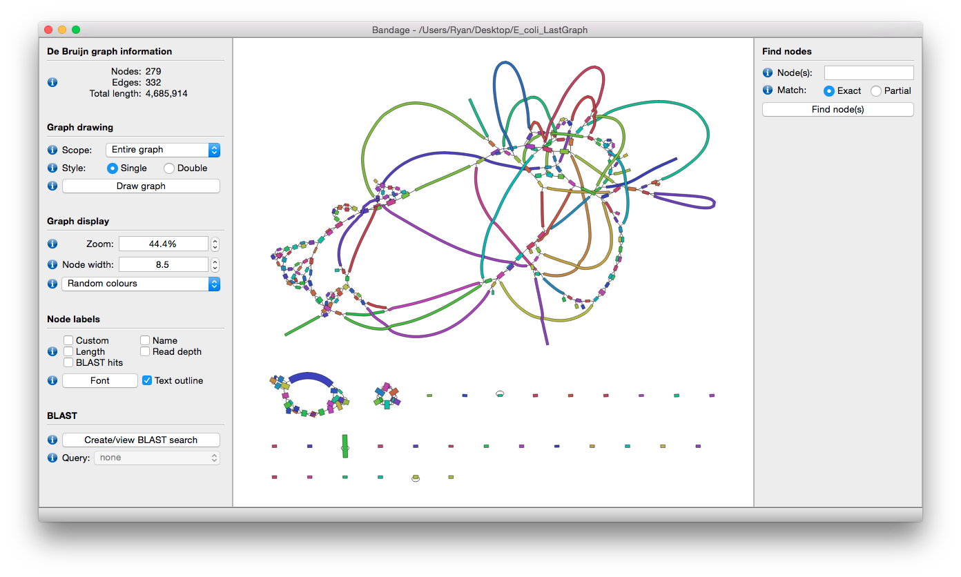
Assignment
Please upload Bandage output