Introduction of R & R plotting II
Ph.D. Tong Zhou
Tong Zhou, Ph.D.
L-207B, Center for Molecular Medicine, MS575
Department of Physiology and Cell Biology
University of Nevada, Reno School of Medicine
1664 North Virginia Street, Reno , NV 89557
The Zhou Lab carries out translational and theoretical research in bioinformatics and computational biology. Much of our research addresses questions of computational molecular medicine and molecular evolution, in particular about the use of genomic data to understand the pathobiology and develop biomarkers for human diseases and to understand the mechanism of exnoic sequence evolution.
Introduction to R
R (www.r-project.org) is a commonly used free Statistics software. R allows you to carry out statistical analyses in an interactive mode, as well as allowing simple programming.

Prepare your laptop
Open two terminal
Connect one to pronghorn
ssh <yourID>@pronghorn.rc.unr.edu
R Installation
Prepare working folder in Pronghorn
cd ~/
mkdir r_plot
cd r_plot
wget -O dataset1.txt https://pastebin.com/raw/N5g8bXg6
wget -O dataset2.txt https://pastebin.com/raw/nAMG57Qy
wget -O heart.txt https://pastebin.com/raw/pN4Tjkkp
wget -O liver.txt https://pastebin.com/raw/Df8vh0Gz
conda activate r_plot
If you missed previous class
cd ~/
mkdir r_plot
cd r_plot
wget -O r_plot.yaml https://pastebin.com/raw/kSAC1AsK
conda env create -n r_plot -f r_plot.yaml
conda activate r_plot
Download results to your laptop
Try this on your laptop
###Please replace <YOURID> to your id.
scp <YOURID>@pronghorn.rc.unr.edu:~/r_plot/*.pdf .
Start R
R
Introduction of R & R plotting – part 2
Matrix
- matrix() function
- Taking the data you input and the number of rows you input (nrow) and making a matrix by filling down each column from the left to the right
matrix(c(1, 2, 3, 4, 5, 6, 7, 8, 9), nrow = 3) - Making a matrix by specifying the number of columns (ncol)
matrix(1:8, ncol = 2) - If there are more elements than data provided
matrix(1:8, nrow=4, ncol = 5)Matrix operations
 #Adding, subtracting, multiplying, and dividing matrices
 m1 = matrix(1:9, ncol=3)
 m1 + 2
 m1 - 10
 m2 = matrix(1:6, ncol=2)
 m2 * 3
 m2 / 2
 m1 + m1
 m1 + m2
 m1 *m1
 m1 / m1
 m1 %*% m2	#Return the inner product
- Taking the data you input and the number of rows you input (nrow) and making a matrix by filling down each column from the left to the right
Matrix manipulation
m = matrix(1:9, ncol=3)
m[1,3]			#Access the element in row 1/column 3
m[2,]			#Access row 2
m[,3]			#Access column 3
m[,-2]			#Remove column 2
m[-1,]			#Remove row 1
m[2,3] = 100			#Change the value in row 2/column 3
m[,1] = 200			#Change the value in column 1
m[,2:3] = 201:206		#Change the value in column 2 and 3
m = matrix(1:50, ncol=5)
#We asked R to give us all the values of matrix  _m_  which had values greater than 5, and it returned these values as a mathematical vector
m[m>25]
m[m>25] = -1		 #change all the values in m that are greater than 5 to -1
Several useful functions
-
colSums()
-
rowSums()
-
colMeans()
-
rowMeans()
m = matrix(seq(1, 1000, by=5), ncol=5)
rowMeans(m)
colMeans(m)
rowSums(m)
colSums(m)
Exercise
Generate a matrix with elements from 1 to 80 (10 rows and 8 columns)
m = matrix(1:80, nrow=10)
Change the values in the matrix that are divisible by 3 or 7 to 100
m[m%%3==0 | m%%7==0] = 100
Pick up the rows with row mean > 70
m[rowMeans(m)>70,]
Data frame
-
May be regarded as a matrix with columns possibly of differing modes and attributes
-
May be displayed in matrix form, and its rows and columns can be extracted using matrix indexing conventions
#Create a data frame
#We have 20 mouse lung tissue samples
#10 from wildtype (WT) mice and 10 from Mylk knockout (KO) mice
#We also know the expression of two Mylk-related genes
sample = c(rep("WT", 10), rep("KO", 10))
gene1 = rnorm(20, mean=5, sd=1)	#rnorm: generate numbers from a normal distribution
gene2 = rnorm(20, mean=15, sd=3)
data = data.frame(sample, gene1, gene2)
Data frame manipulation
#Show column names
colnames(data)
#Use dolloar sign $ to access a column
data$sample
data$gene2
#Pick up the samples with gene1 expression > 5 and gene2 expression <15
data[data$gene1 > 5 & data$gene2 <15,]
#Add a new column to the data frame
gene3 = rnorm(20, mean=2, sd=0.3)
data = data.frame(data, gene3)
#Plot a boxplot showing the difference in gene1 expression between the WT and KO samples
pdf(file="boxplot_gene1.pdf", width=3, height=4)
boxplot(data$gene1 ~ data$sample, col=c("grey40", "grey80"), xlab="", ylab="Expression")
dev.off()
Read a data frame from file
#Load the human subject data sheet: dataset2.txt
#52 subject: 16 healthy controls and 36 patientth glioma
data = read.delim("dataset2.txt")
data
#Use the function table() to count at eacmbination of factor levels
table(data$Type)
table(data$Sex)
table(data$Type, data$Sex)
#Split the data according to subject type anmpute the mean age for each
aggregate(data$Age~data$Type, FUN=mean)
#Plot a boxplot showing the difference in agtween the control and glioma groups
pdf(file="boxplot_age1.pdf", width=3, height=4)
boxplot(data$Age ~ data$Type, col=c("grey80","orange"), xlab="", ylab="Age")
dev.off()
Exercise
Extract the female subjects with age>50
data[data$Sex == "F" & data&Age>50,]
Plot a boxplot showing the group difference in age among the male subjects
data[data$Sex=="F" & data$Age>50,]
pdf(file="boxplot_age2.pdf", width=3, height=4)
male = data[data$Sex=="M",]
boxplot(male$Age ~ male$Type)
dev.off()
#Alternative solution
pdf(file="boxplot_age2.pdf", width=3, height=4)
boxplot(data$Age[data$Sex=="M"] ~ data$Type[data$Sex=="M"])
dev.off()
R plotting
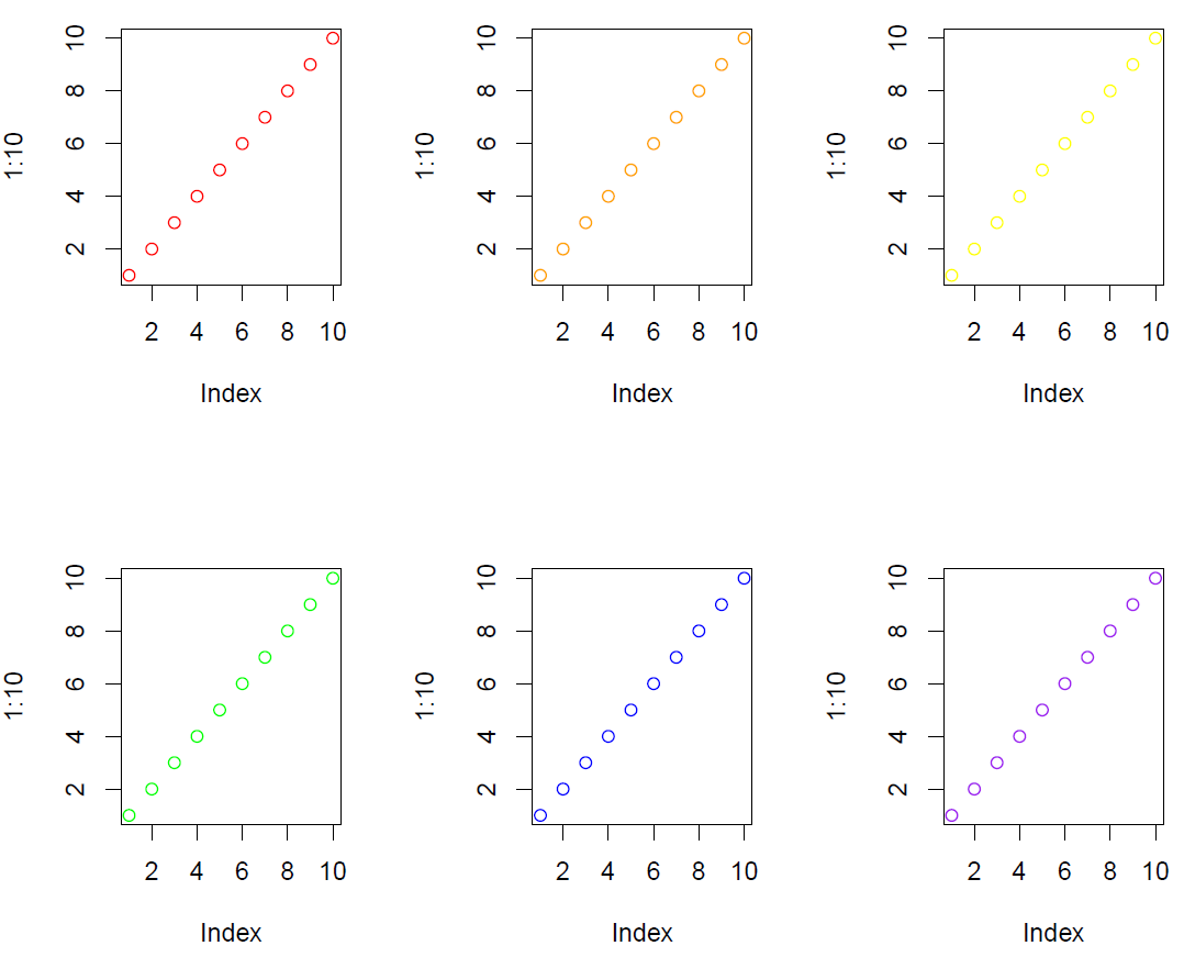
Split display and plot figures
 pdf(file="split_screen.pdf", width=8, height=7)
 split.screen(c(2, 3))	# split display into six sreens
 screen(1)		# prepare screen 1 for output
 plot(1:10, col="red")
 screen(2)		# prepare screen 2 for output
 plot(1:10, col="orange")
 screen(3)		# prepare screen 3 for output
 plot(1:10, col="yellow")
 screen(4)		# prepare screen 4 for output
 plot(1:10, col="green")
 screen(5)		# prepare screen 5 for output
 plot(1:10, col="blue")
 screen(6)		# prepare screen 6 for output
 plot(1:10, col="purple")
 close.screen(all = TRUE)	# exit split-screen mode
 dev.off()
Dataset “Dataset1.txt”
- Boxplots for TP63 and SLC2A1
#1 load the expression data sheet - 78 samples and  72 genes
expr = read.delim("dataset1.txt", row.names="gene")
#2 the first 30 samples are normal lung tissue while the last 48 samples are from lung tumors
cl = c(rep("Normal", 30), rep("Tumor", 48))
#3 boxplot showing the difference in expression of 63 and SLC2A1 between normal and tumor tissues
pdf(file="boxplot_two_genes.pdf", width=6, height=4)
split.screen(c(1, 3))
screen(1)
boxplot(t(expr["TP63",])~cl, xlab="", ylab="Expression", main="TP63", col=c("grey80", "orange"), xaxt="n")
screen(2)
boxplot(t(expr["SLC2A1",])~cl, xlab="", ylab="Expression", main="SLC2A1", col=c("grey80", "orange"), xaxt="n")
screen(3)
legend("left", fill=c("grey80", "orange"), c("Normal", "Tumor"), bty="n")
close.screen(all = TRUE)
dev.off()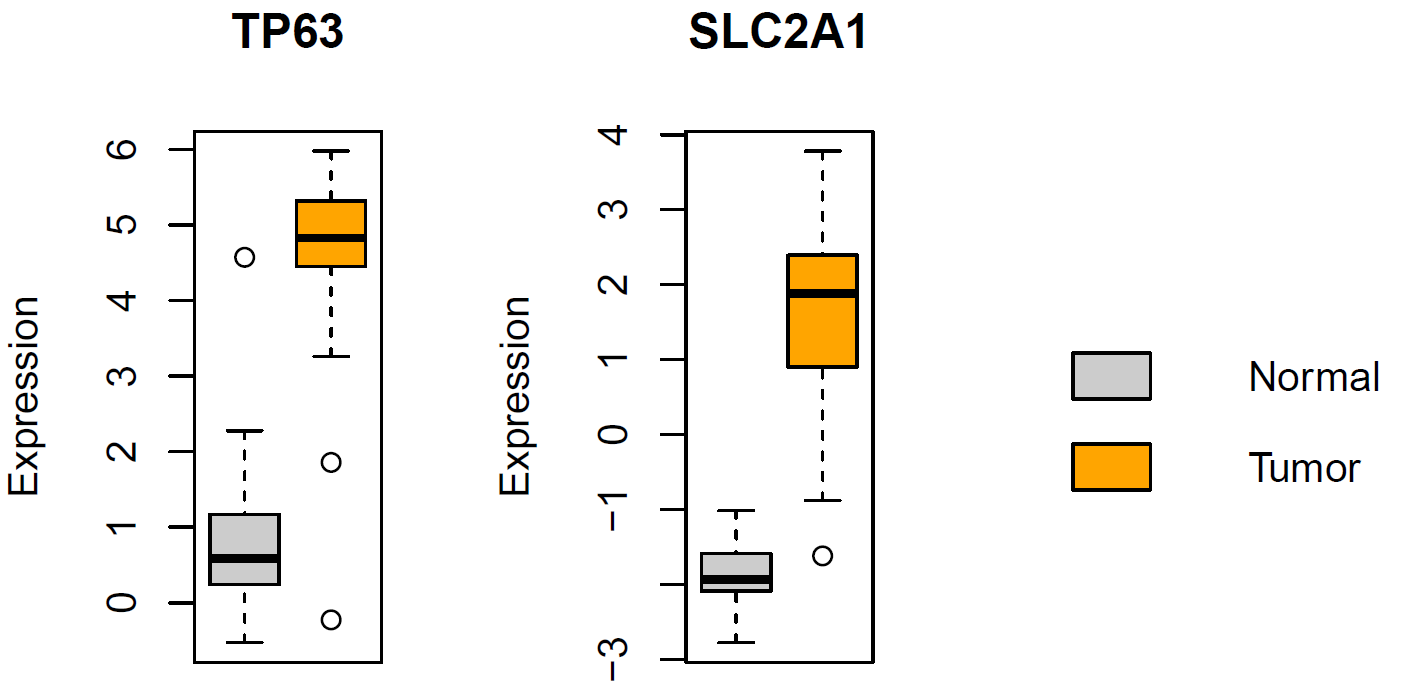
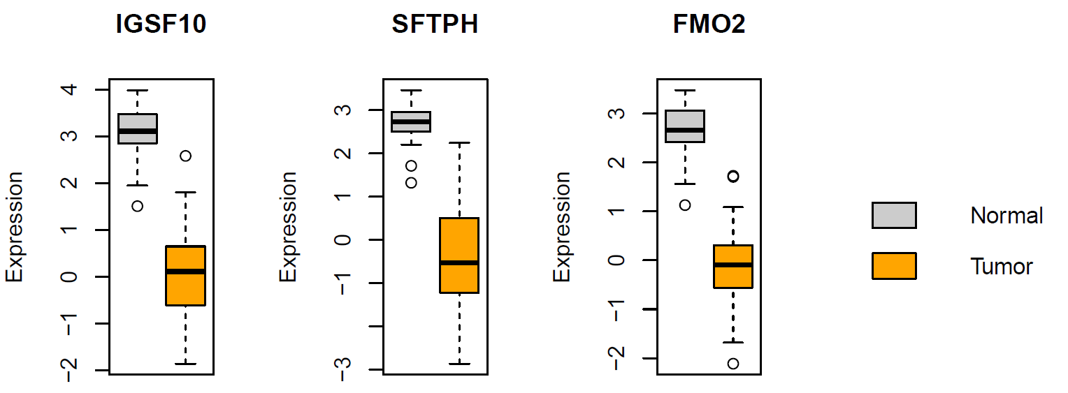
Exercise
Based on “dataset1.txt”, generate boxplots showing the difference in expression of IGSF10 , SFTPH , and FMO2 between normal and tumor tissues
# boxplot showing the difference in expression of IGSF10, SFTPH, and FMO2 between normal and tumor tissues
pdf(file="boxplot_three_genes.pdf", width=8, height=4)
split.screen(c(1, 4))
screen(1)
boxplot(t(expr["IGSF10",])~cl, xlab="", ylab="Expression", main="IGSF10", col=c("grey80", "orange"), xaxt="n")
screen(2)
boxplot(t(expr["SFTPH",])~cl, xlab="", ylab="Expression", main="SFTPH", col=c("grey80", "orange"), xaxt="n")
screen(3)
boxplot(t(expr["FMO2",])~cl, xlab="", ylab="Expression", main="FMO2", col=c("grey80", "orange"), xaxt="n")
screen(4)
legend("left", fill=c("grey80", "orange"), c("Normal", "Tumor"), bty="n")
close.screen(all = TRUE)
dev.off()
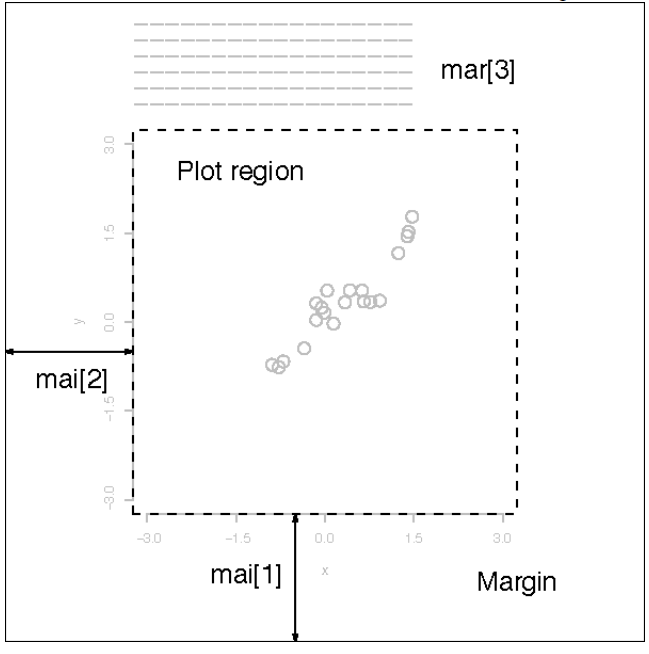
par()
- Build-in function par() can be used to set graphical parameters
- mai: a numerical vector of the form c(bottom, left, top, right) which gives the margin size specified in inches
- tck: the length of tick marks
- cex.main: the size to be used for main titles
- font.main: the font to be used for main titles
- mgp: the location for the axis labels, tick mark labels, and tick marks relative to the plot
Dataset “heart.txt”
Load the “heart.txt” dataset
expr = read.delim("heart.txt", row.names="gene")
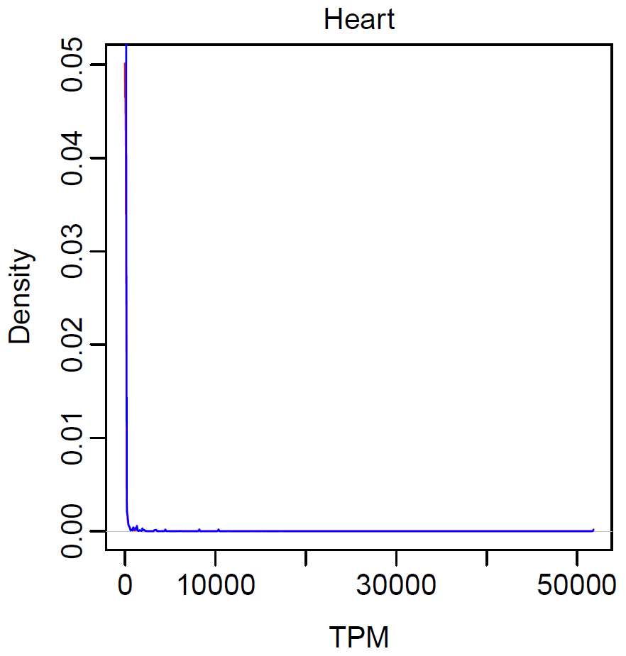
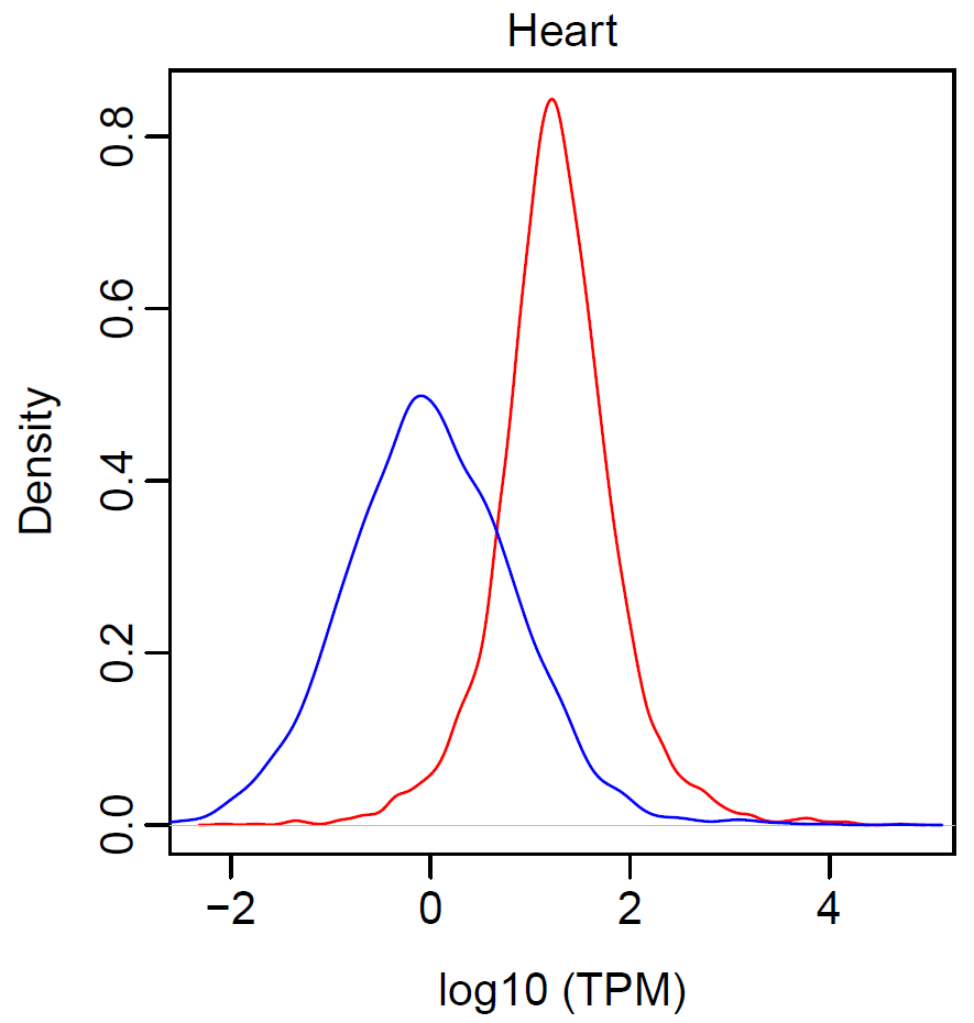
- Distribution in expression of the linear/circular transcripts in heart
pdf(file="expression_distribution1.pdf", width=4, height=4) par(mai=c(0.8, 0.8, 0.3, 0.3), mgp=c(2, 0.5, 0), tck=-0.03, cex.main=1, font.main=1) plot(density(expr$linear), col="red", main="Heart", xlab="TPM", ylab="Density") lines(density(expr$circular), col="blue") dev.off()pdf(file="expression_distribution2.pdf", width=4, height=4) par(mai=c(0.8, 0.8, 0.3, 0.3), mgp=c(2, 0.5, 0), tck=-0.03, cex.main=1, font.main=1) plot(density(log10(expr$linear)), col="red", main="Heart", xlab="log10 (TPM)", ylab="Density") lines(density(log10(expr$circular)), col="blue") dev.off()
- Test relationship between linear and circular transcripts in heart
cor.test(expr$linear, expr$circular)
cor.test(expr$linear, expr$circular, method="spearman")
 pdf(file="correlation_heart.pdf", width=4, height=4)
par(mai=c(0.8, 0.8, 0.3, 0.3), mgp=c(2, 0.5, 0), tck=-0.03, cex.main=1, font.main=1)
plot(log10(expr$linear), log10(expr$circular), xlim=c(-4, 4), ylim=c(-4, 4), col="grey70", pch=20, cex=0.5, xlab=expression(paste("Mean ", TPM[linear])), ylab=expression(paste("Mean ", TPM[circ])), main="Heart", axes=F)
lines(lowess(log10(expr$linear), log10(expr$circular), f=1/3), col="red", lty=1)
abline(a=0, b=1, lty=2)
axis(1, at=-2:2*2, c(expression(10^-4), expression(10^-2), 1, expression(10^2), expression(10^4)), cex.axis=1)
axis(2, at=-2:2*2, c(expression(10^-4), expression(10^-2), 1, expression(10^2), expression(10^4)), cex.axis=1)
dev.off()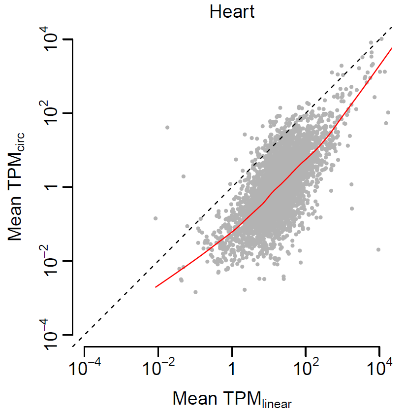
#Linear regression
relation = lm(log10(expr$circular)~log10(expr$linear))
summary(relation)
pdf(file="linear_regression_heart.pdf", width=4, height=4, useDingbats=FALSE)
par(mai=c(0.8, 0.8, 0.3, 0.3), mgp=c(2, 0.5, 0), tck=-0.03, cex.main=1, font.main=1)
plot(log10(expr$linear), log10(expr$circular), xlim=c(-4, 4), ylim=c(-4, 4), col="grey70", pch=20, cex=0.5, xlab=expression(paste("Mean ", TPM[linear])), ylab=expression(paste("Mean ", TPM[circ])), main="Heart", axes=F)
abline(lm(log10(expr$circular)~log10(expr$linear)), col="red")
abline(a=0, b=1, lty=2)
axis(1, at=-2:2*2, c(expression(10^-4), expression(10^-2), 1, expression(10^2), expression(10^4)), cex.axis=1)
axis(2, at=-2:2*2, c(expression(10^-4), expression(10^-2), 1, expression(10^2), expression(10^4)), cex.axis=1)
dev.off()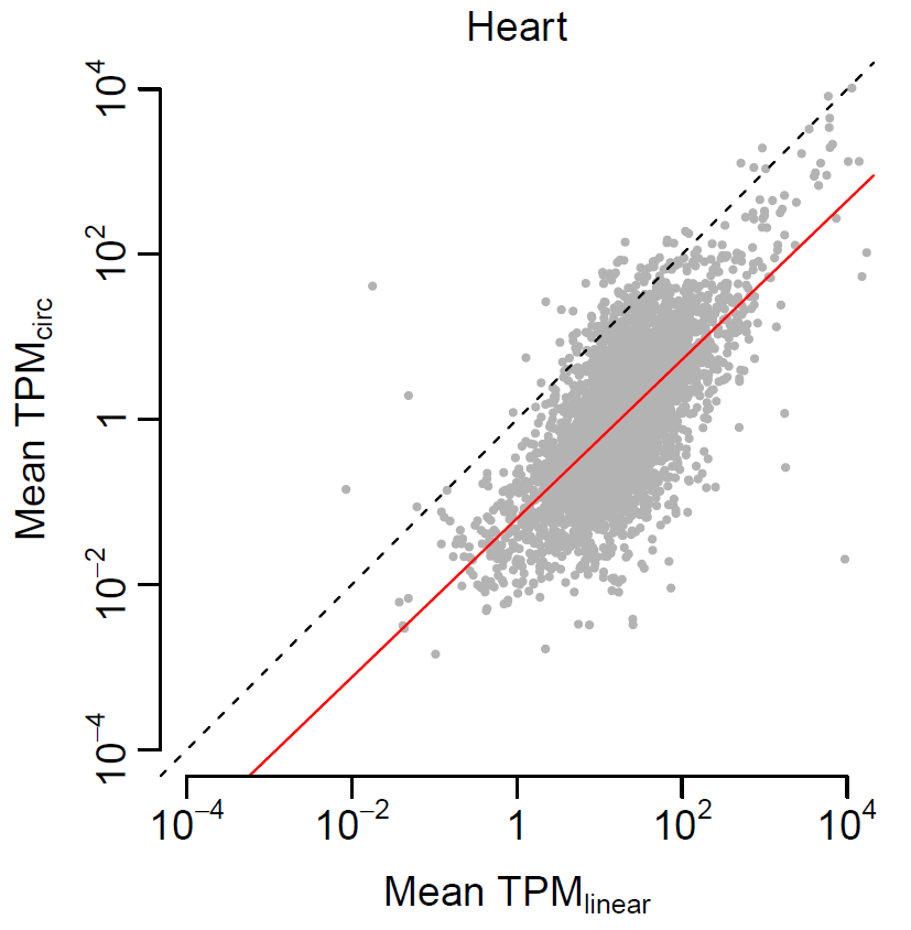
Exercise
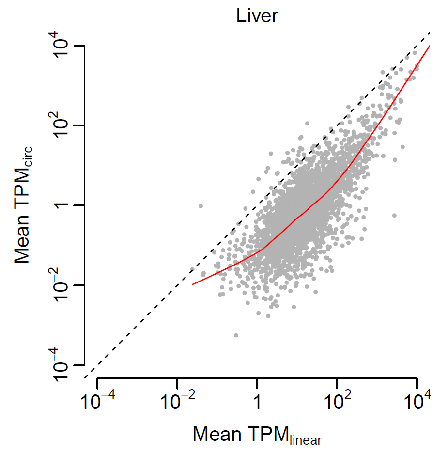
- Test the correlation in expression between linear and circular transcripts in liver
- Read the data frame from “liver.txt“
- Plot the distribution of the linear/circular RNA expression
- Perform Pearson/Spearman correlation test in expression between linear and circular transcripts
- Plot the correlation in expression between linear and circular transcripts in liver
Solution
#Correlation in expression between linear and circular transcripts in liver expr = read.delim("liver.txt", row.names="gene") pdf(file="expression_distribution3.pdf", width=4, height=4) par(mai=c(0.8, 0.8, 0.3, 0.3), mgp=c(2, 0.5, 0), tck=-0.03, cex.main=1, font.main=1) plot(density(log10(expr$linear)), col="red", main="Liver", xlab="log10 (TPM)", ylab="Density") lines(density(log10(expr$circular)), col="blue") dev.off()cor.test(expr$linear, expr$circular) cor.test(expr$linear, expr$circular, method="spearman") pdf(file="correlation_liver.pdf", width=4, height=4, useDingbats=FALSE) par(mai=c(0.8, 0.8, 0.3, 0.3), mgp=c(2, 0.5, 0), tck=-0.03, cex.main=1, font.main=1) plot(log10(expr$linear), log10(expr$circular), xlim=c(-4, 4), ylim=c(-4, 4), col="grey70", pch=20, cex=0.5, xlab=expression(paste("Mean ", TPM[linear])), ylab=expression(paste("Mean ", TPM[circ])), main="Liver", axes=F) lines(lowess(log10(expr$linear), log10(expr$circular), f=1/3), col="red", lty=1) abline(a=0, b=1, lty=2) axis(1, at=-2:2*2, c(expression(10^-4), expression(10^-2), 1, expression(10^2), expression(10^4)), cex.axis=1) axis(2, at=-2:2*2, c(expression(10^-4), expression(10^-2), 1, expression(10^2), expression(10^4)), cex.axis=1) dev.off()
Contact information
Email: tongz@med.unr.edu
If you have any question, please contact me by email.
Reading materials
The R Project for Statistical Computing https://www.r-project.org/
R Graphic cookbook https://learning.oreilly.com/library/view/r-graphics-cookbook/9781491978597/
R workshop https://bioinformatics.ca/workshops/2018-introduction-to-R/
RStudio https://www.rstudio.com/
Wikipedia R (programming language) https://en.wikipedia.org/wiki/R_(programming_language)
Wikipedia RStudio https://en.wikipedia.org/wiki/RStudio