Genome assembly
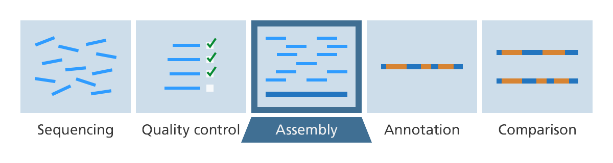
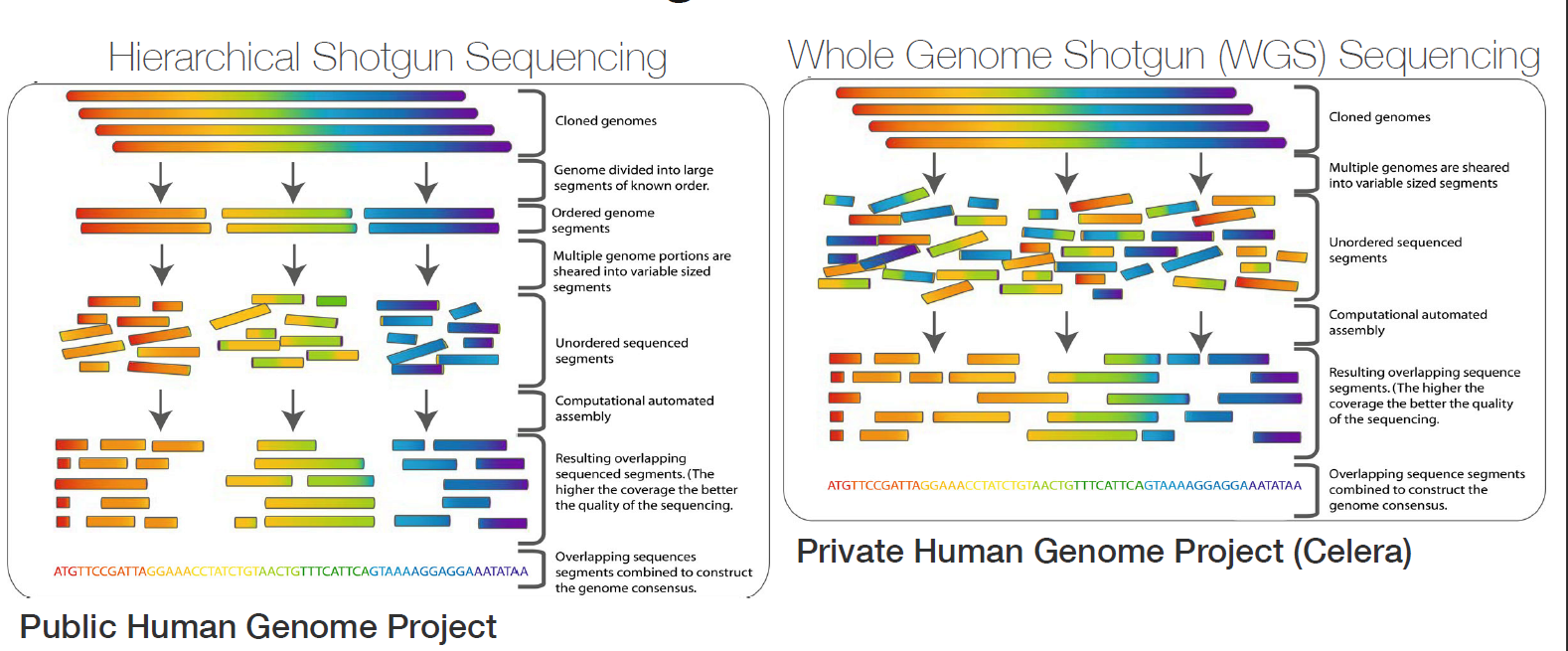
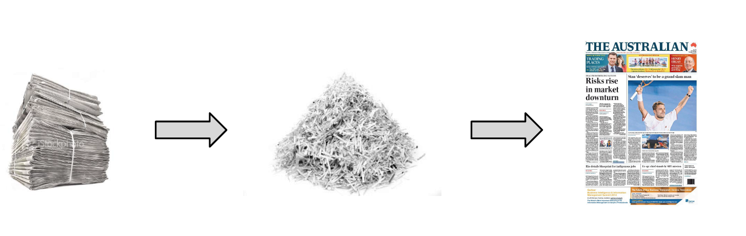
After DNA sequencing is complete, the fragments of DNA that come out of the machine are all jumbled up. Like a jigsaw puzzle we need to take the pieces of the genome and put them back together.
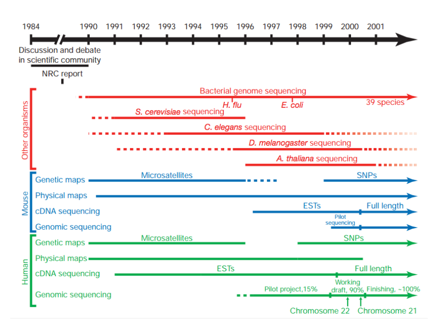
The human genome required a significant technological push
25✕ larger than any previously sequenced genome
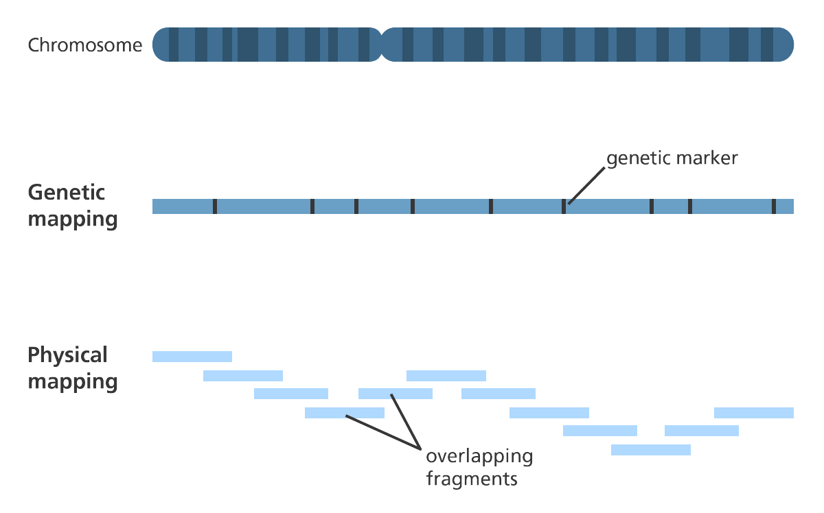
- Construction of genetic and physical maps of human and mouse genomes
- Sequencing of yeast and worm genomes
- Pilot projects to test the feasibility and cost effectiveness of large-scale sequencing
What’s the challenge?
-
The technology of DNA sequencing? is not 100 per cent accurate and therefore there are likely to be errors in the DNA sequence that is produced.
-
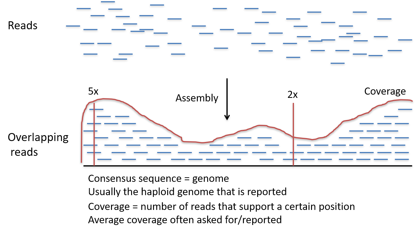
So, to account for the errors that could potentially occur, each base in the genome? is sequenced a number of times over, this is called coverage. For example, 30 times (30-fold) coverage means each base? is sequenced 30 times.
-
Effectively, the more times you sequence, or
read, the same section of DNA, the more confidence you have that the final sequence is correct. 30- to 50-fold coverage is currently the standard used when sequencing human genomes to a high level of accuracy. -
During the Human Genome Project? coverage was only between 5- and 10-fold and used a different sequencing technology to those used today.
-
Coverage has increased because of a few reasons: Although most current sequencing techniques are now faster than they were during the Human Genome Project, some sequencing technologies have a higher error rate. Some sequencing technologies deal with shorter reads of DNA which means that gaps are more likely to occur when the genome is assembled. Having a higher coverage reduces the likelihood of there being gaps in the final assembled sequence. It is also much cheaper to carry out sequencing to a higher coverage than it was at the time of the Human Genome Project.
-
High coverage means that after sequencing DNA we have lots and lots of pieces of DNA sequence (reads).
-
To put this into perspective, once a human genome has been fully sequenced we have around 100 gigabases (100,000,000,000 bases) of sequence data.
-
Like the pieces of a jigsaw puzzle, these DNA reads are jumbled up so we need to piece them together and put them in the correct order to assemble the genome sequence.
Coverage calculation
Example: I know that the genome size. I am sequencing 10 Mbases genome species. I want a 50x coverage to do a good assembly. I am ordering 125 bp Illumina reads. How many reads do I need?
- (125xN)/10e+6=50
- N=(50x10e+6)/125=4e+6 (4 million reads)
De novo assembly
-
De novo sequencing is when the genome of an organism is sequenced for the first time.
- In de novo assembly there is no existing reference genome sequence for that species to use as a template for the assembly of its genome sequence.
- If you know that the new species? is very similar to another species that does have a reference genome, it is possible to assemble the sequence using a similar genome as a guide.
- To help assemble a de novo sequence a physical gene? map can be developed before sequencing to highlight the landmarks so the scientists know where sections of DNA are located in relation to each other.
- Producing a gene map can be an expensive process, so some assembly programmes rely on data consisting of a mix of single and paired-end reads
-
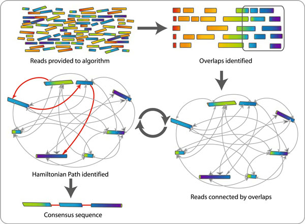
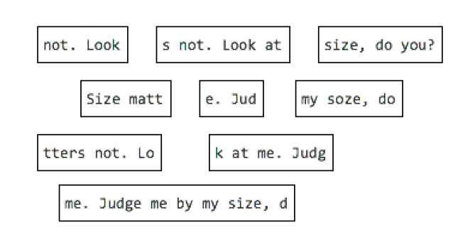
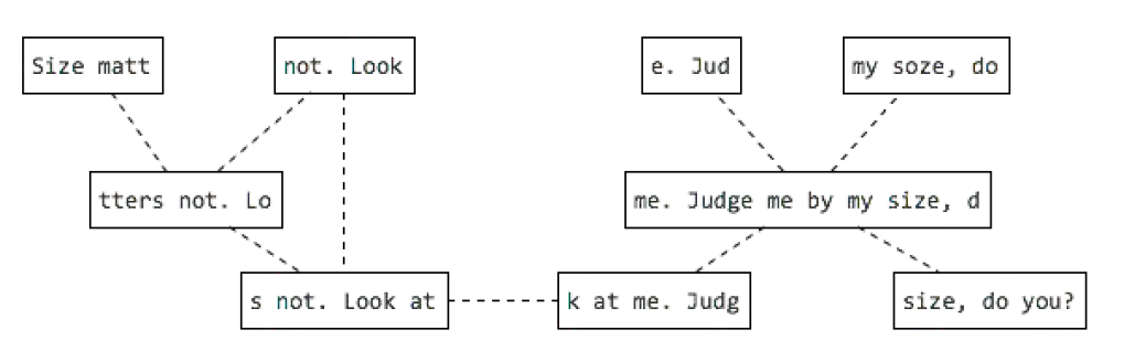
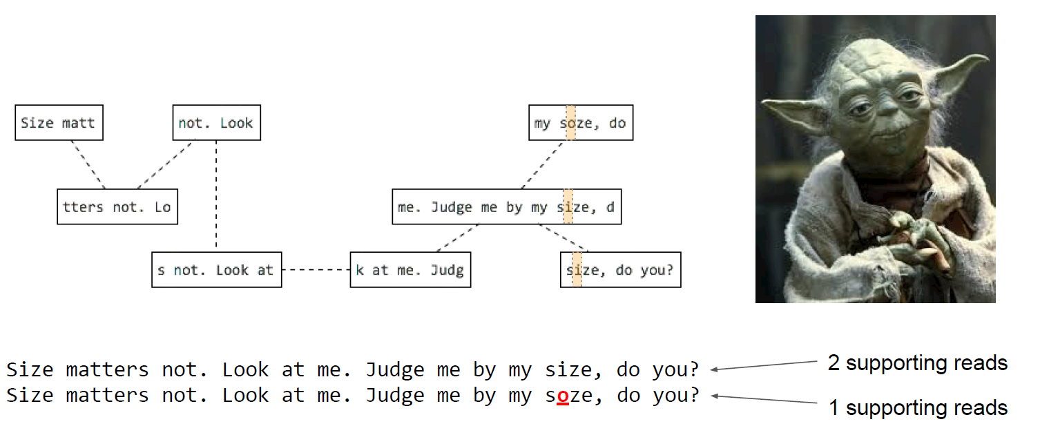
Single reads are where one end or the whole of a fragment of DNA is sequenced. These sequences can then be joined together by finding overlapping regions in the sequence to create the full DNA sequence.
-
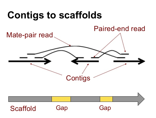
Paired-end reads are where both ends of a fragment of DNA are sequenced. The distance between paired-end reads can be anywhere between 200 base pairs? and several thousand. The key advantage of paired-end reads is that scientists know how far apart the two ends are. This makes it easier to assemble them into a continuous DNA sequence. Paired-end reads are particularly useful when assembling a de novo sequence as they provide long-range information that you wouldn’t otherwise have in the absence of a gene map.
- Assembly of a de novo sequence begins with a large number of short sections or “reads” of DNA.
- These reads are compared to each other and those sharing the same DNA sequence are grouped together.
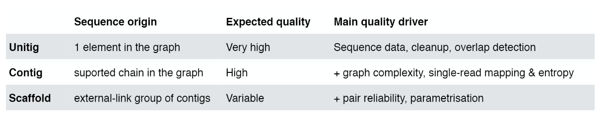
- From here they are assembled into progressively larger sections to form long contiguous (together in sequence) sequences called “contigs”.
- These contigs can then be grouped together with information taken from other technologies to provide clues for how to stitch the contigs together and roughly how far apart to place them, even if the sequence in between is still unknown. This is called “scaffolding”.
- The assembly can be further refined by ordering the individual scaffolds into chromosomes?. A physical gene map is a useful tool for doing this.
- The resulting assembly is then fed on to the next stage of the process – annotation, which identifies where the genes and other features in the sequence start and stop.
- The assembly of a genome is a computer-intensive job. It usually takes around 20 hours per gigabase of sequence for genome assembly programmes to stitch together an organism’s genome sequence from the reads of DNA sequence generated by the sequencing machines.
- So, with the 100 gigabases of sequence data we have after sequencing a human genome, it will take 2,000 hours or around 83 days to assemble the complete sequence.
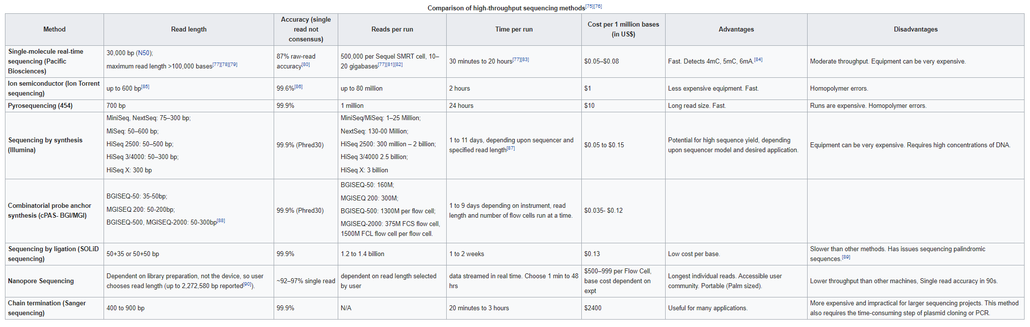
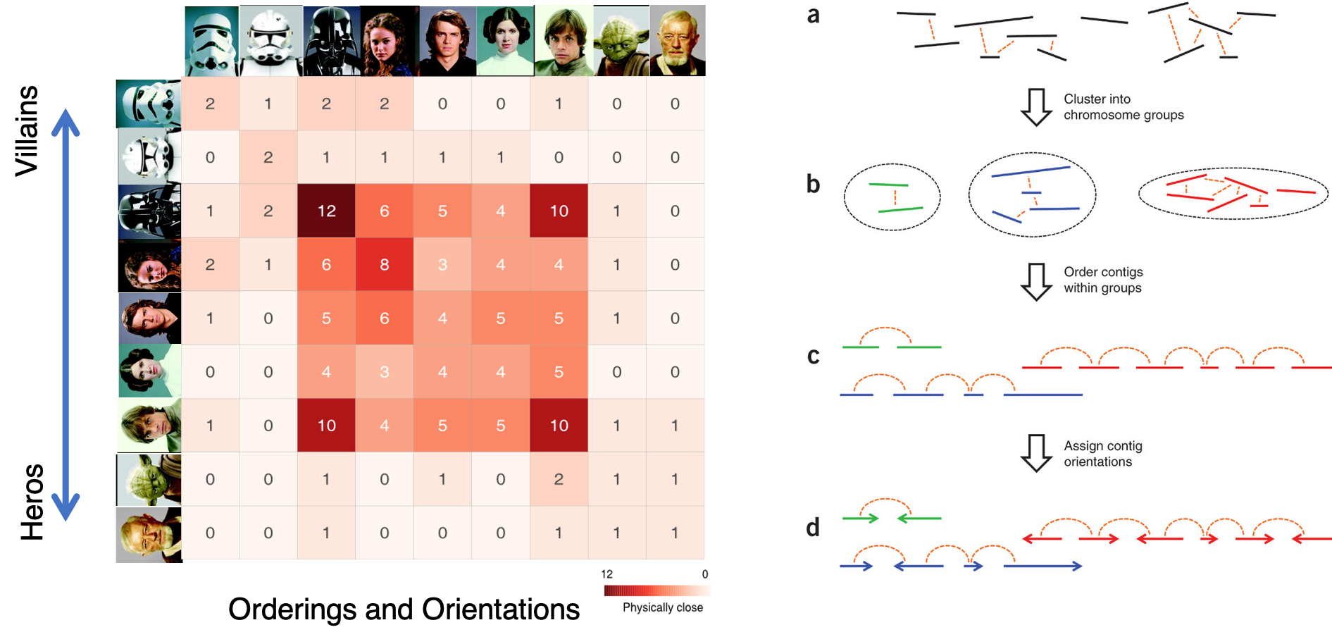
Genome assembly refers to the process of taking a large number of short DNA sequences and putting them back together to create a representation of the original chromosomes from which the DNA originated. De novo genome assemblies assume no prior knowledge of the source DNA sequence length, layout or composition. In a genome sequencing project, the DNA of the target organism is broken up into millions of small pieces and read on a sequencing machine. These “reads” vary from 20 to 1000 nucleotide base pairs (bp) in length depending on the sequencing method used. Typically for Illumina type short read sequencing, reads of length 36 - 150 bp are produced. These reads can be either single ended as described above or paired end. A good summary of other types of DNA sequencing can be found below.
Paired end reads are produced when the fragment size used in the sequencing process is much longer (typically 250 - 500 bp long) and the ends of the fragment are read in towards the middle. This produces two “paired” reads. One from the left hand end of a fragment and one from the right with a known separation distance between them. (The known separation distance is actually a distribution with a mean and standard deviation as not all original fragments are of the same length.) This extra information contained in the paired end reads can be useful for helping to tie pieces of sequence together during the assembly process.
The goal of a sequence assembler is to produce long contiguous pieces of sequence (contigs) from these reads. The contigs are sometimes then ordered and oriented in relation to one another to form scaffolds. The distances between pairs of a set of paired end reads is useful information for this purpose.
The mechanisms used by assembly software are varied but the most common type for short reads is assembly by de Bruijn graph. See this document for an explanation of the de Bruijn graph genome assembler “SPAdes.”
Genome assembly is a very difficult computational problem, made more difficult because many genomes contain large numbers of identical sequences, known as repeats. These repeats can be thousands of nucleotides long, and some occur in thousands of different locations, especially in the large genomes of plants and animals.
Why do we want to assemble an organism’s DNA?
Determining the DNA sequence of an organism is useful in fundamental research into why and how they live, as well as in applied subjects. Because of the importance of DNA to living things, knowledge of a DNA sequence may be useful in practically any biological research. For example, in medicine it can be used to identify, diagnose and potentially develop treatments for genetic diseases. Similarly, research into pathogens may lead to treatments for contagious diseases.
What do we need to do?
- Put the pieces together in the correct order to construct the complete genome sequence and identify any areas of interest.
-
This is done using processes called alignment and assembly:
Alignment is when the new DNA sequence is compared to existing DNA sequences to find any similarities or discrepancies between them and then arranged to show these features. Alignment is a vital part of assembly.Assembly involves taking a large number of DNA reads, looking for areas in which they overlap with each other and then gradually piecing together the ‘jigsaw’. It is an attempt to reconstruct the original genome. This is primarily carried out for de novo sequences?.
The protocol in a nutshell:
- Obtain sequence read file(s) from sequencing machine(s).
- Look at the reads - get an understanding of what you’ve got and what the quality is like.
- Raw data cleanup/quality trimming if necessary.
- Choose an appropriate assembly parameter set.
- Assemble the data into contigs/scaffolds.
- Examine the output of the assembly and assess assembly quality.
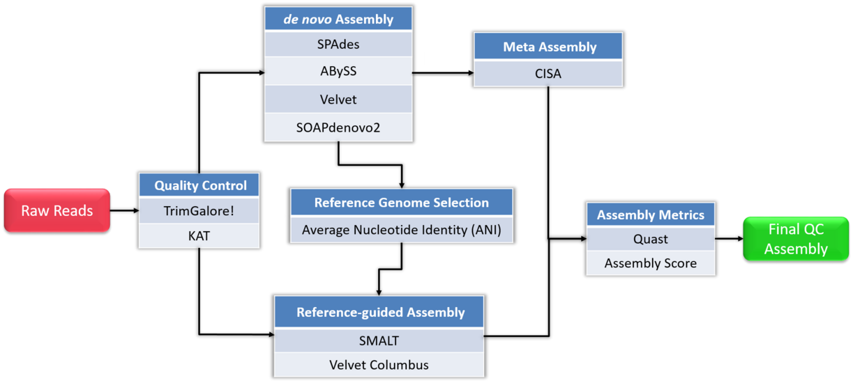
Flowchart of de novo assembly protocol.
Long read sequencing
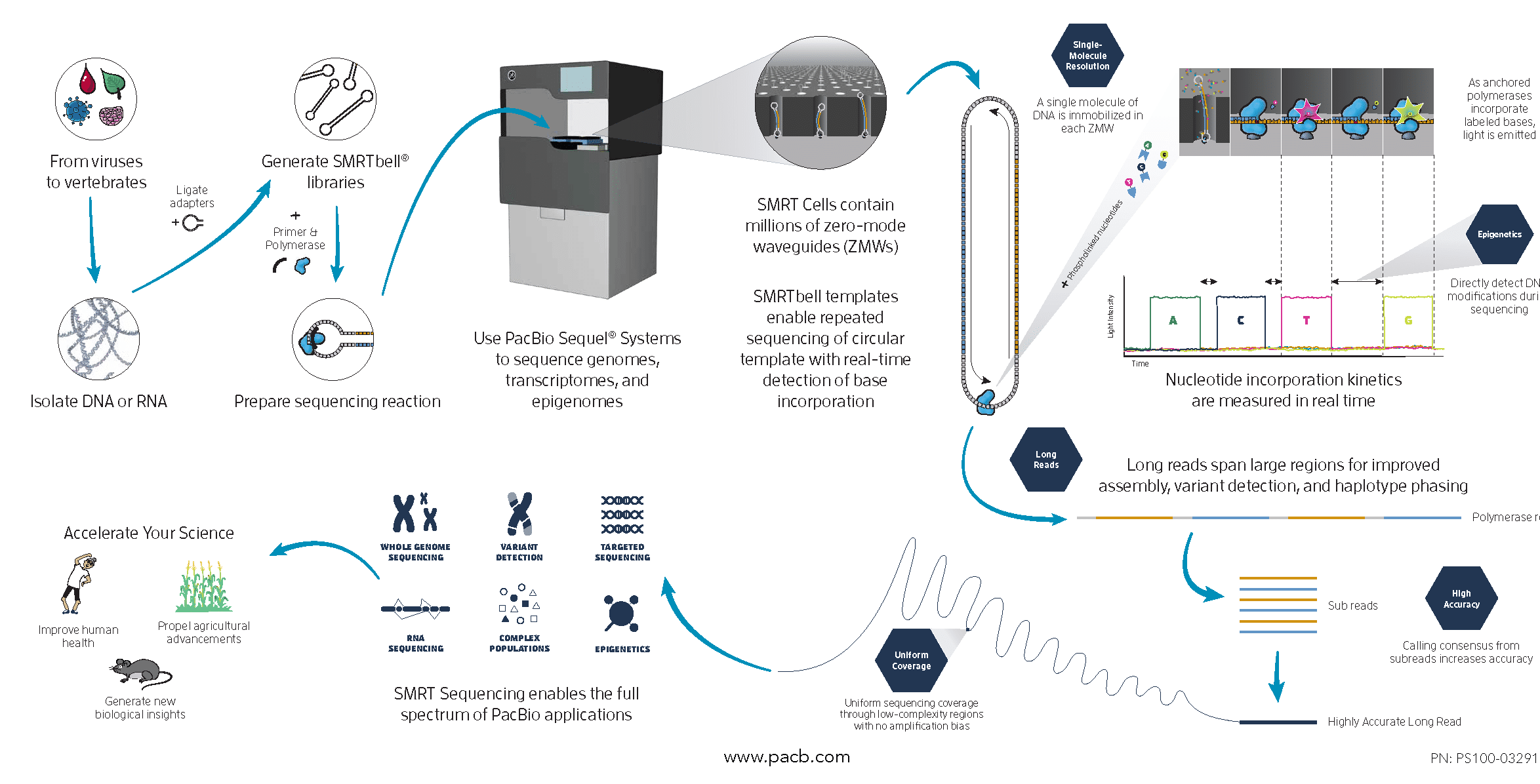
Single Molecule, Real-Time (SMRT) Sequencing is the core technology powering our long-read sequencing platforms. This innovative approach was the first of its kind and is now a proven technology used in all fields of life science.
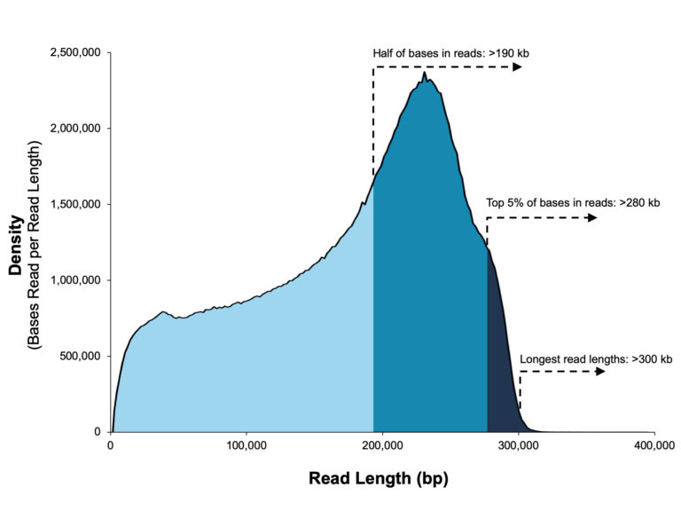
Long Reads (PacBio)
With reads tens of kilobases in length you can readily assemble complete genomes and sequence full-length transcripts.
 A 20 kb size-selected human library using the SMRTbell Express Template Prep Kit 2.0 on a Sequel II System (2.0 Chemistry, Sequel II System Software v8.0, 30-hour movie).
SMRT Sequencing enables simultaneous collection of data from millions of wells using the natural process of DNA replication to sequence long fragments of native DNA or RNA.
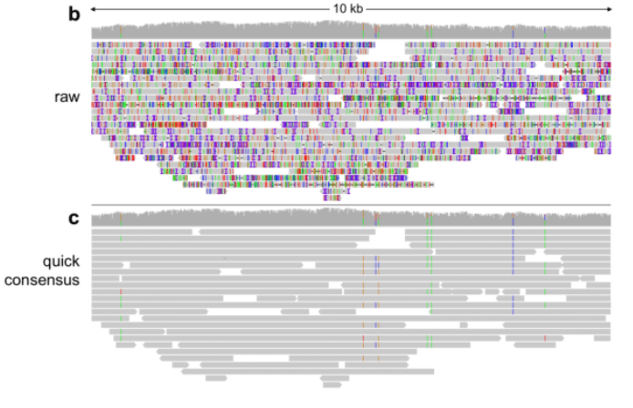
PacBio Error
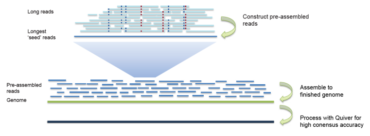
Long Reads Assembly
OLC Algorithm
OLC example
Long reads publications
- Mitsuhashi, Satomi et al. (2019) Long-read sequencing for rare human genetic diseases. Journal of human genetics
- Wenger, Aaron M et al. (2019) Accurate circular consensus long-read sequencing improves variant detection and assembly of a human genome. Nature biotechnology
- Eichler, Evan E et al. (2019) Genetic Variation, Comparative Genomics, and the Diagnosis of Disease. The New England journal of medicine
- Mantere, Tuomo et al. (2019) Long-Read Sequencing Emerging in Medical Genetics Frontiers in genetics
- Wang, Bo et al. (2019) Reviving the Transcriptome Studies: An Insight into the Emergence of Single-molecule Transcriptome Sequencing Frontiers in genetics
- Pollard, Martin O et al. (2018) Long reads: their purpose and place. Human molecular genetics
- Sedlazeck, Fritz J et al. (2018) Accurate detection of complex structural variations using single-molecule sequencing. Nature methods
- Ardui, Simon et al. (2018) Single molecule real-time (SMRT) sequencing comes of age: applications and utilities for medical diagnostics. Nucleic acids research
- Nakano, Kazuma et al. (2017) Advantages of genome sequencing by long-read sequencer using SMRT technology in medical area. Human cell
- Chaisson, Mark J P et al. (2015) Genetic variation and the de novo assembly of human genomes. Nature reviews. Genetics
- Rhoads, Anthony et al. (2015) PacBio sequencing and its applications. Genomics, proteomics & bioinformatics
- Berlin, Konstantin et al. (2015) Assembling large genomes with single-molecule sequencing and locality-sensitive hashing. Nature biotechnology
- Huddleston, John et al. (2014) Reconstructing complex regions of genomes using long-read sequencing technology. Genome research
- Koren, Sergey et al. (2013) Reducing assembly complexity of microbial genomes with single-molecule sequencing. Genome biology
- Travers, Kevin J et al. (2010) A flexible and efficient template format for circular consensus sequencing and SNP detection. Nucleic acids research
- Flusberg, Benjamin A et al. (2010) Direct detection of DNA methylation during single-molecule, real-time sequencing. Nature methods
- Eid, John et al. (2009) Real-time DNA sequencing from single polymerase molecules. Science
Repeat in Genome
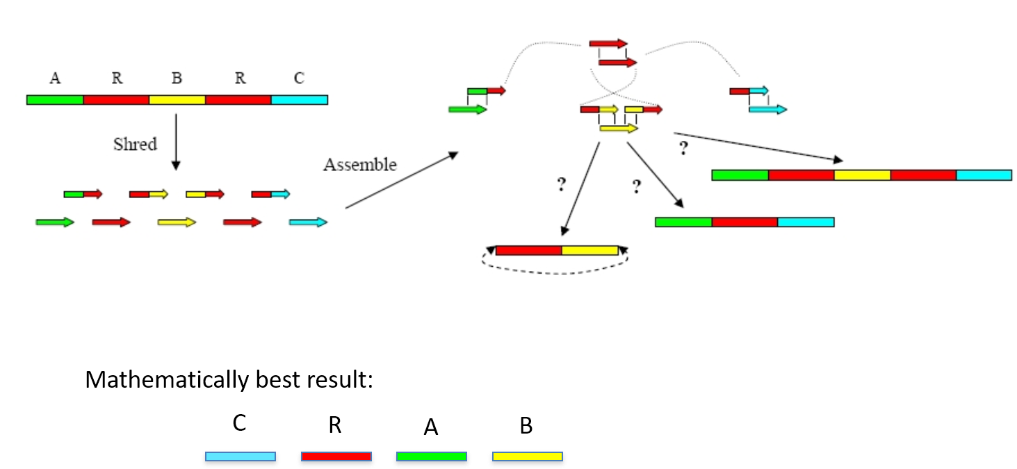
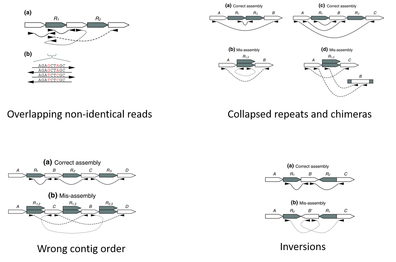
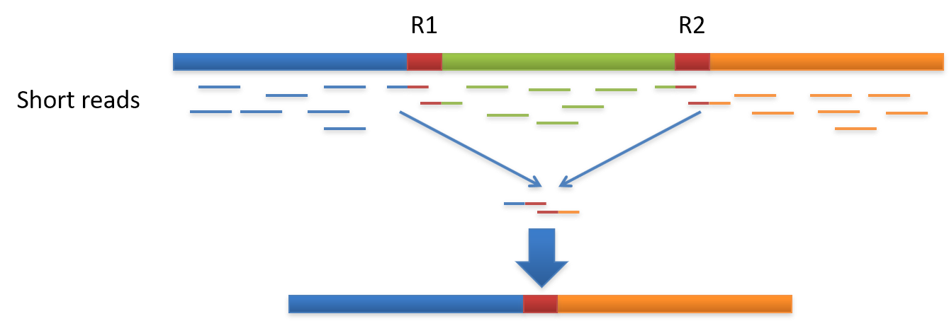
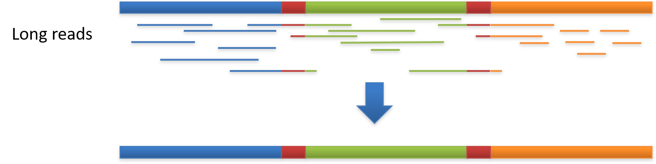
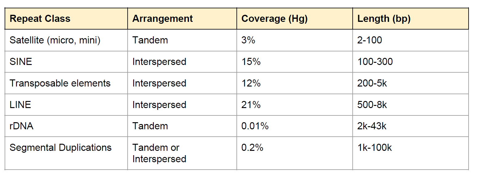
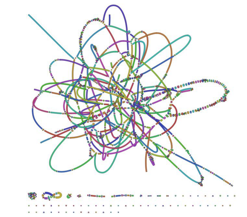 Fig: E.coli genome (4.6Mbp)
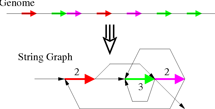
String Graph Algorithm
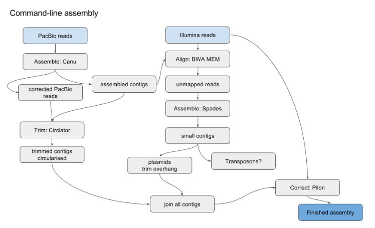
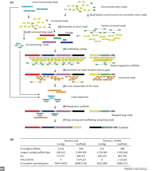
Hybrid Assembly
Genome assembly complexity
GC-content
- Regions of low or high GC-content have a lower coverage (Illumina, not PacBio)
Secondary structure
- Regions that are tightly bound get less coverage
Ploidy level
- On higher ploidy levels you potentially have more alleles present
Size of organism
- Hard to extract enough DNA from small organisms
Pooled individuals
- Increases the variability of the DNA (more alleles)
Inhibiting compounds
- Lower coverage and shorter fragments
Presence of additional genomes/contamination
- Lower coverage of what you actually are interested in, potentially chimeric assemblies
Heterozygosity
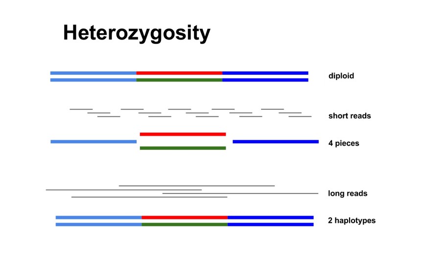
Haplotype
Contiguity
- Fewer contigs
- Longer contigs
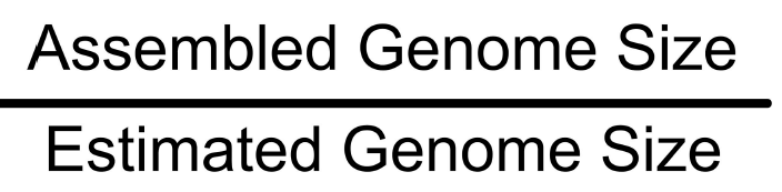
Completeness : Total size
Proportion of the original genome represented by the assembly Can be between 0 and 1
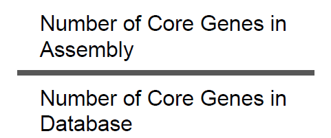
Completeness: core genes
-
Proportion of coding sequences can be estimated based on known core genes thought to be present in a wide variety of organisms.
-
Assumes that the proportion of assembled genes is equal to the proportion of assembled core genes.
Correctness
Proportion of the assembly that is free from errors
Errors include
- Mis-joins
- Repeat compressions
- Unnecessary duplications
- Indels / SNPs caused by assembler
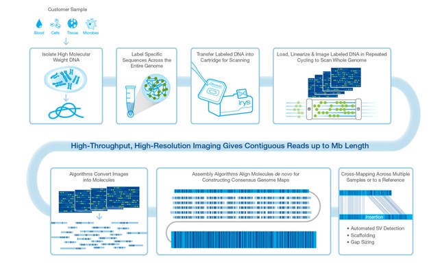
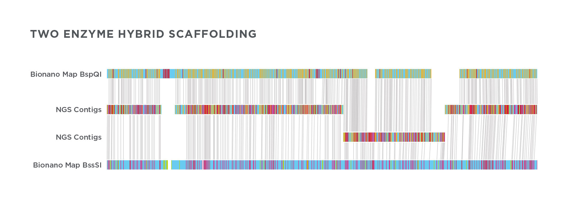
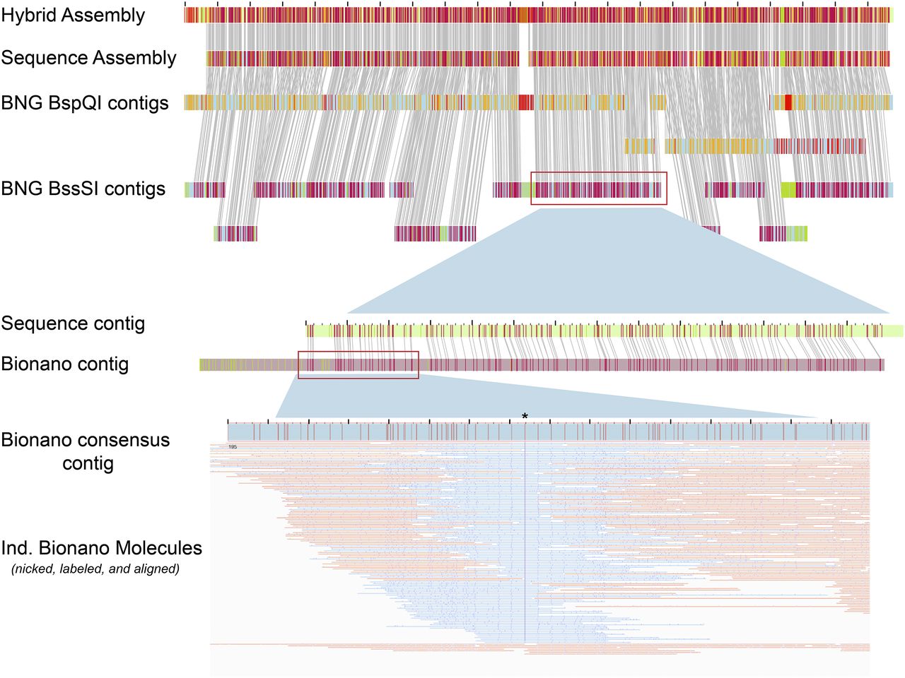
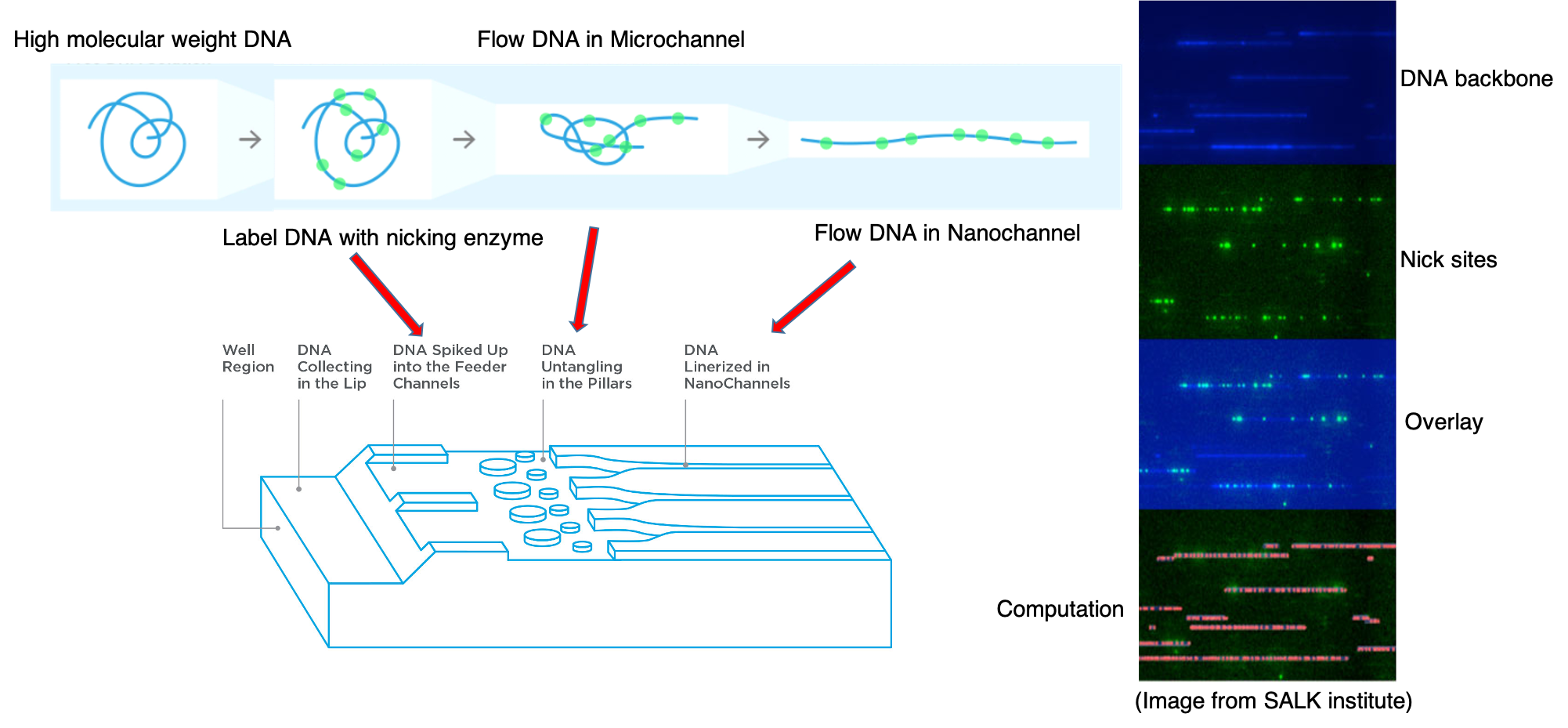
Optical mapping
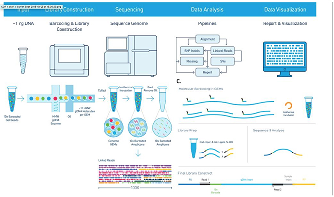
10x Genomics
Assembly results
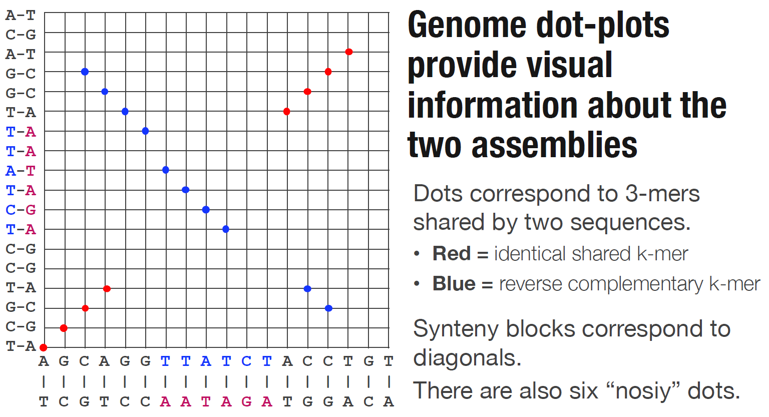
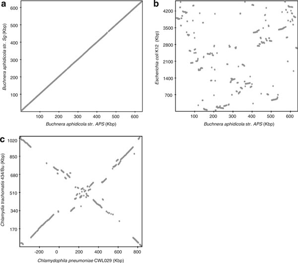
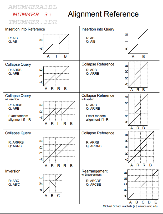
Dotplot
Metrics
- Number of contigs
- Average contig length
- Median contig length
- Maximum contig length
- “N50”, “NG50”, “D50”
Assembly statistics
N50

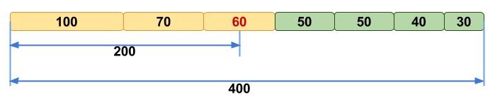
N50 example
N50 is a measure to describe the quality of assembled genomes that are fragmented in contigs of different length. The N50 is defined as the minimum contig length needed to cover 50% of the genome.
| Contig Length |
|---|
| 100 |
| 200 |
| 230 |
| 400 |
| 750 |
| 852 |
| 950 |
| 990 |
| 1020 |
| 1278 |
| 1280 |
| 1290 |
N50 example
| Contig Length | Cumulative Sum |
|---|---|
| 100 | 100 |
| 200 | 300 |
| 230 | 530 |
| 400 | 930 |
| 750 | 1680 |
| 852 | 2532 |
| 950 | 3482 |
| 990 | 4472 |
| 1020 | 5492 |
| 1278 | 6770 |
| 1280 | 8050 |
| 1290 | 9340 |
Why assemble genomes
- Produce a reference for new species
- Genomic variation can be studied by comparing against the reference
- A wide variety of molecular biological tools become available or more effective
- Coding sequences can be studied in the context of their related non-coding (eg regulatory) sequences
- High level genome structure (number, arrangement of genes and repeats) can be studied
Assembly is very challenging (“impossible”) because
- Sequencing bias under represents certain regions
- Reads are short relative to genome size
- Repeats create tangled hubs in the assembly graph
- Sequencing errors cause detours and bubbles in the assembly graph
Prerequisite
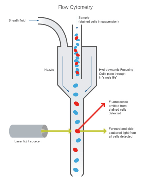
Flow Cytometry
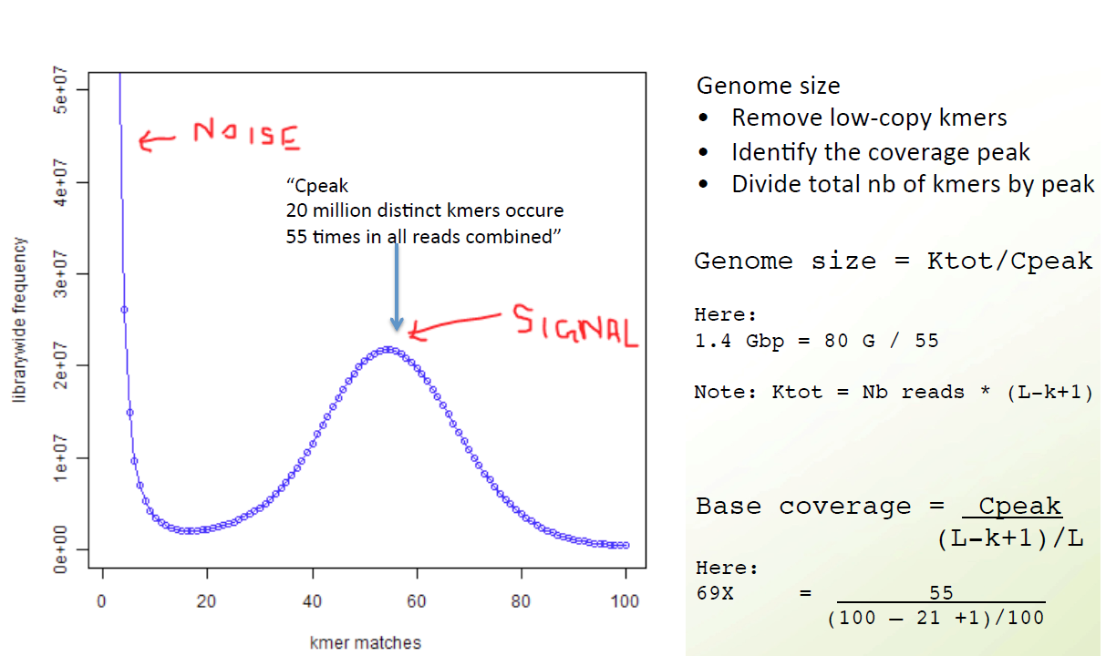
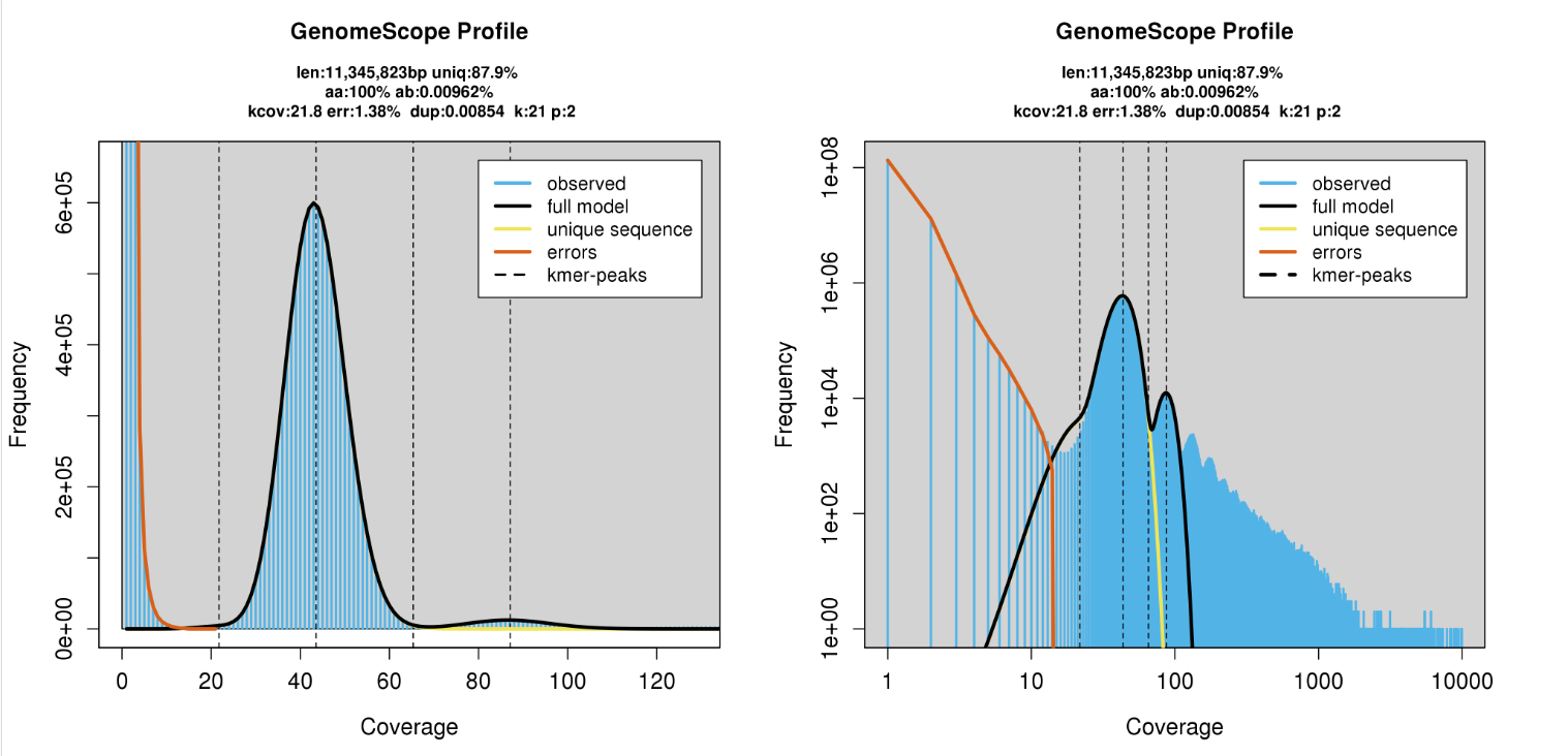
K-mer spectrum
How can we improve these genome assemblies?
Mate Pair Sequencing
BioNano Optical Mapping
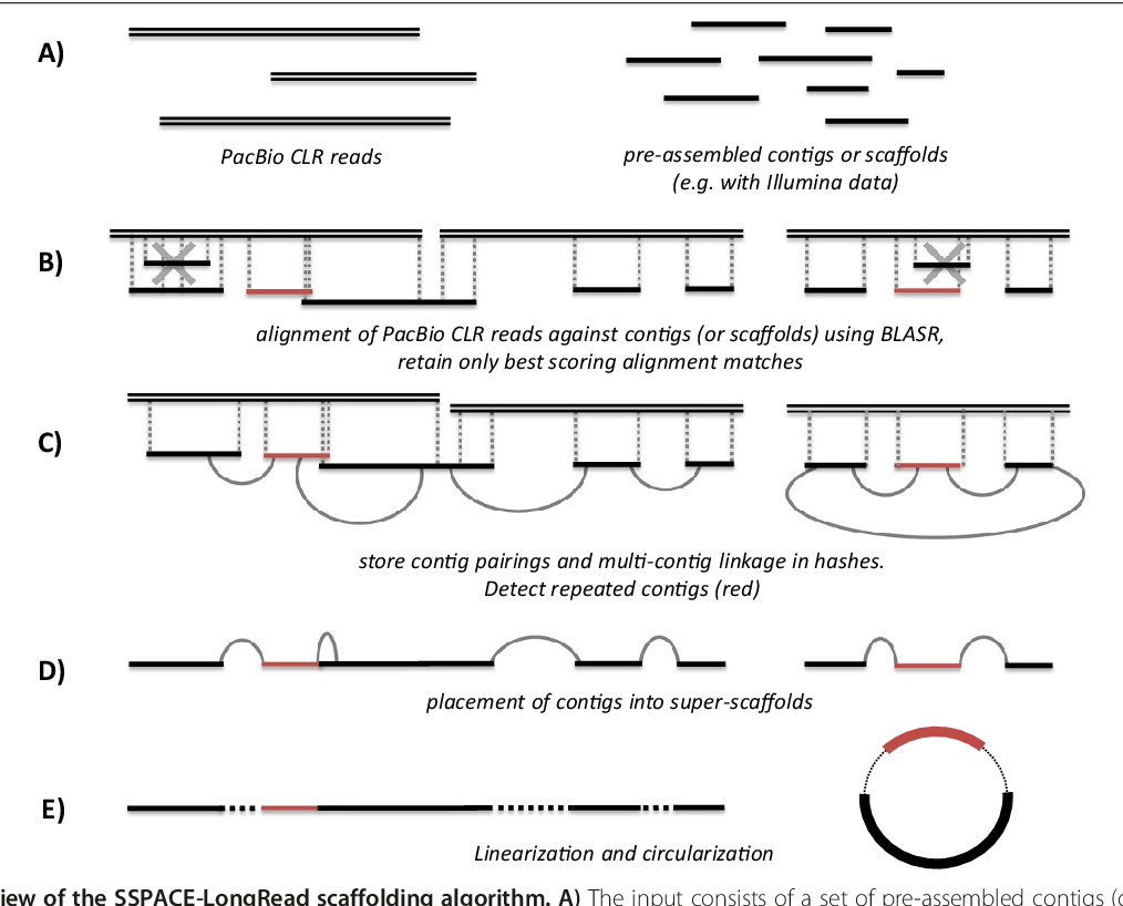
Long Read Scaffolding
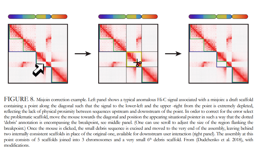
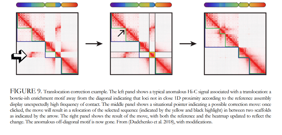
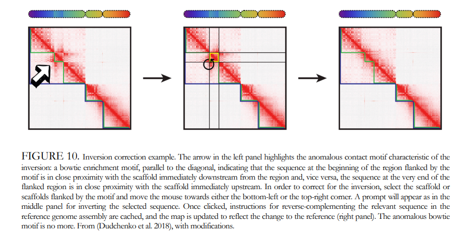
Chromosome Conformation Scaffolding
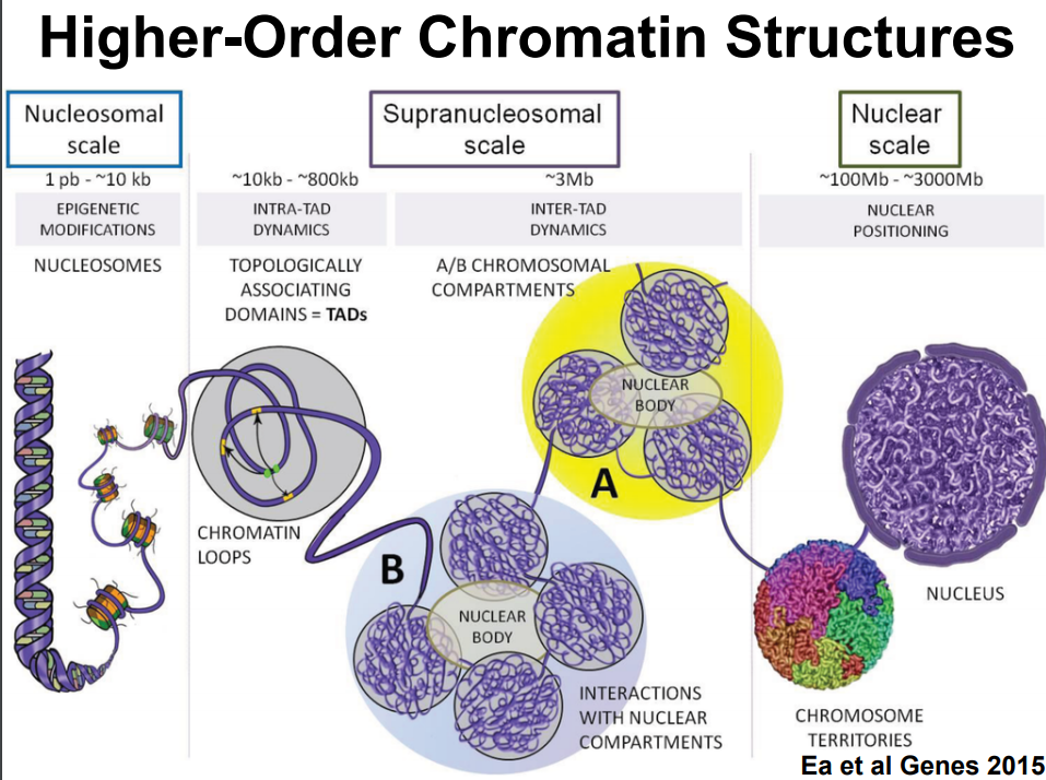
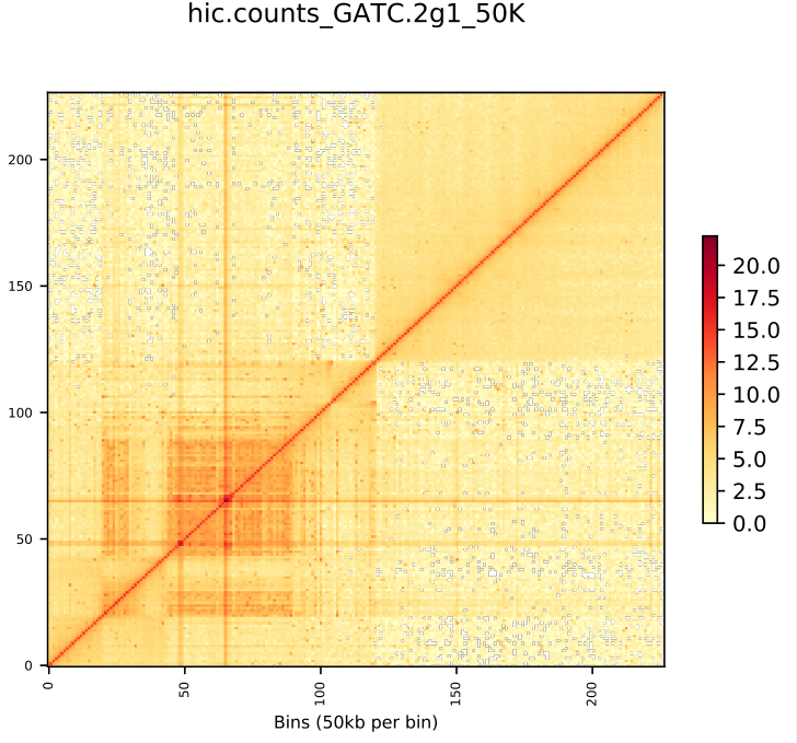
HiC for Genome Assembly
ALLHiC
Phasing and scaffolding polyploid genomes based on Hi-C data
Introduction
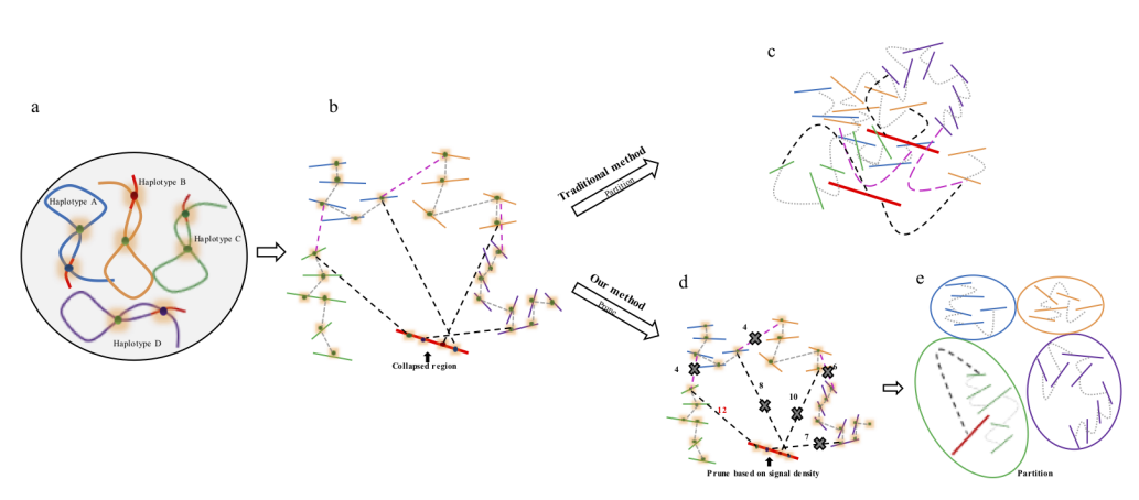
The major problem of scaffolding polyploid genome is that Hi-C signals are frequently detected between allelic haplotypes and any existing stat of art Hi-C scaffolding program links the allelic haplotypes together. To solve the problem, we developed a new Hi-C scaffolding pipeline, called ALLHIC, specifically tailored to the polyploid genomes. ALLHIC pipeline contains a total of 5 steps: prune, partition, rescue, optimize and build.
Overview of ALLHiC

Figure 1. Overview of major steps in ALLHiC algorithm. The newly released ALLHiC pipeline contains a total of 5 functions: prune, partition, rescue, optimize and build. Briefly, the prune step removes the inter-allelic links so that the homologous chromosomes are more easily separated individually. The partition function takes pruned bam file as input and clusters the linked contigs based on the linkage suggested by Hi-C, presumably along the same homologous chromosome in a preset number of partitions. The rescue function searches for contigs that are not involved in partition step from original un-pruned bam files and assigned them to specific clusters according Hi-C signal density. The optimize step takes each partition, and optimize the ordering and orientations for all the contigs. Finally, the build step reconstructs each chromosome by concatenating the contigs, adding gaps between the contigs and generating the final genome release in FASTA format.
Explanation of Prune
Prune function will firstly allow us to detect allelic contigs, which can be achieved by identifying syntenic genes based on a well-assembled close related species or an assembled monoploid genome. Signals (normalized Hi-C reads) between allelic contigs are removed from the input BAM files. In polyploid genome assembly, haplotypes that share high similarity are likely to be collapsed. Signals between the collapsed regions and nearby phased haplotypes result in chimeric scaffolds. In the prune step, only the best linkage between collapsed coting and phased contig is retained.
 Figure 2. Description of Hi-C scaffolding problem in polyploid genome and application of prune approach for haplotype phasing. (a) a schematic diagram of auto-tetraploid genome. Four homologous chromosomes are indicated as different colors (blue, orange, green and purple, respectively). Red regions in the chromosomes indicate sequences with high similarity. (b) Detection of Hi-C signals in the auto-tetraploid genome. Black dash lines indicate Hi-C signals between collapsed regions and un-collpased contigs. Pink dash lines indicate inter-haplotype Hi-C links and grey dash lines indicate intra-haplotype Hi-C links. During assembly, red regions will be collapsed due to high sequence similarity; while, other regions will be separated into different contigs if they have abundant variations. Since the collapsed regions are physically related with contigs from different haplotypes, Hi-C signals will be detected between collapsed regions with all other un-collapsed contigs. (c) Traditional Hi-C scaffolding methods will detect signals among contigs from different haplotypes as well as collapsed regions and cluster all the sequences together. (d) Prune Hi-C signals: 1- remove signals between allelic regions; 2- only retain the strongest signals between collapsed regions and un-collapsed contigs. (e) Partition based on pruned Hi-C information. Contigs are ideally phased into different groups based on prune results.
Citations
Zhang, X. Zhang, S. Zhao, Q. Ming, R. Tang, H. Assembly of allele-aware, chromosomal scale autopolyploid genomes based on Hi-C data. Nature Plants, doi:10.1038/s41477-019-0487-8 (2019).
Zhang, J. Zhang, X. Tang, H. Zhang, Q. et al. Allele-defined genome of the autopolyploid sugarcane Saccharum spontaneum L. Nature Genetics, doi:10.1038/s41588-018-0237-2 (2018).
Algorithm demo
Solving scaffold ordering and orientation (OO) in general is NP-hard. ALLMAPS converts the problem into Traveling Salesman Problem (TSP) and refines scaffold OO using Genetic Algorithm. For rough idea, a ‘live’ demo of the scaffold OO on yellow catfish chromosome 1 can be viewed in the animation below.

Traveling Salesman Problem
Allhic result
DOT plot
https://dnanexus.github.io/dot/
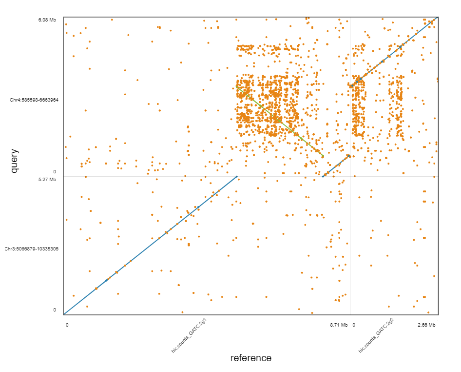
What is the problem?
Genome Annotation
After the sections of DNA sequence have been assembled into a complete genome sequence we need to identify where the genes and key features are. We have our aligned and assembled genome sequence but how do we identify where the genes and other functional regions of the genome are located.
-
Annotation involves marking where the genes start and stop in the DNA sequence and also where other relevant and interesting regions are in the sequence.
-
Although genome annotation pipelines can differ from one another, for example, some elements can be manual while others have to be automated, they all share a core set of features.
-
They are generally divided into two distinct phases: gene prediction and manual annotation.
Gene prediction
There are two types of gene prediction: Ab initio – this technique relies on signals within the DNA sequence. It is an automated process whereby a computer is given instructions for finding genes in the sequence and is then left to find them. The computer looks for common sequences known to be found at the start and end of genes such as promoter sequences (where proteins bind that switch on genes), start codons (where the code for the gene product, RNA ?or protein, starts) and stop codons (where the code for the gene product ends).
Evidence-based
This technique relies on evidence beyond the DNA sequence. It involves gathering various pieces of genetic information from the transcript sequence (mRNA), and known protein sequences of the genome. With these pieces of evidence it is then possible to get an idea of the original DNA sequence by working backwards through transcription? and translation? (reverse transcription/translation). For example, if you have the protein sequence it is possible to work out the family of possible DNA sequences it could be derived from by working out which amino acids? make up the protein and then which combination of codons could code for those amino acids and so on, until you get to the DNA sequence. The information taken from these two prediction methods is then combined and lined up with the sequenced genome.
Key Point
-
Gene annotation is one of the core mechanisms through which we decipher the information that is contained in genome sequences.
-
Gene annotation is complicated by the existence of ‘transcriptional complexity’, which includes extensive alternative splicing and transcriptional events outside of protein-coding genes.
-
The annotation strategy for a given genome will depend on what it is hoped to achieve, as well as the resources available.
-
The availability of next-generation data sets has transformed gene annotation pipelines in recent years, although their incorporation is rarely straightforward.
-
Even human gene annotation is far from complete: transcripts are missing and existing models are truncated. Most importantly, ‘functional annotation’ — the description of what transcripts actually do — remains far from comprehensive.
-
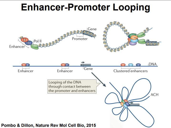
Efforts are now under way to integrate gene annotation pipelines with projects that seek to describe regulatory sequences, such as promoter and enhancer elements.
-
Gene annotation is producing increasingly complex resources. This can present a challenge to usability, most notably in a clinical context, and annotation projects must find ways to resolve such problems.
The core annotation workflows for different gene types.
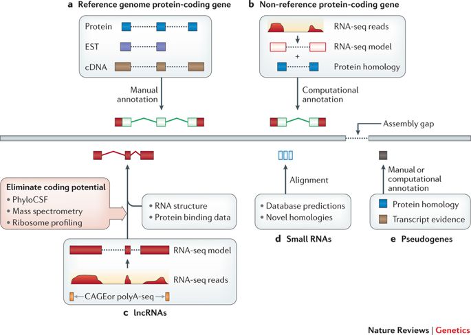
| These workflows illustrate general annotation principles rather than the specific pipelines of any particular genebuild. a | Protein-coding genes within reference genomes were generally annotated on the basis of the computational genomic alignment of Sanger-sequenced transcripts and protein-coding sequences, followed by manual annotation using interface tools such as Zmap, WebApollo, Artemis and the Integrative Genomics Viewer. Transcripts were typically taken from GenBank129 and proteins from Swiss-Prot. b | Protein-coding genes within non-reference genomes are usually annotated based on fewer resources; in this case, RNA sequencing (RNA-seq) data are used in combination with protein homology information that has been extrapolated from a closely related genome. RNA-seq pipelines for read alignment include STAR and TopHat, whereas model creation is commonly carried out by Cufflinks23. c | Long non-coding RNA (lncRNA) structures can be annotated in a similar manner to protein-coding transcripts (parts a and b), although coding potential must be ruled out. This is typically done by examining sequence conservation with PhyloCSF or using experimental data sets, such as mass spectrometry or ribosome profiling. In this example, 5′ Cap Analysis of Gene Expression (CAGE) and polyA-seq data are also incorporated to obtain true transcript end points. Designated lncRNA pipelines include PLAR. d | Small RNAs are typically added to genebuilds by mining repositories such as RFAM or miRBase. However, these entries can be used to search for additional loci based on homology. e | Pseudogene annotation is based on the identification of loci with protein homology to either paralogous or orthologous protein-coding genes. Computational annotation pipelines include PseudoPipe53, although manual annotation is more accurate. Finally, all annotation methods can be thwarted by the existence of sequence gaps in the genome assembly (right-angled arrow). EST, expressed sequence tag. |
High-level strategies for gene annotation projects.
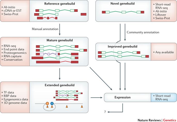
This schematic details the annotation pathways for reference and novel genomes. Coding sequences (CDSs) are outlined in green, nonsense-mediated decay (NMD) is shown in purple and untranslated regions (UTRs) are filled in in red. The core evidence sets that are used at each stage are listed, although their availability and incorporation can vary across different projects. The types of evidence used for reference genebuilds have evolved over time: RNA sequencing (RNA-seq) has replaced Sanger sequencing, conservation-based methodologies have become more powerful and proteogenomic data sets are now available. By contrast, novel genebuilds are constructed based on RNA-seq and/or ab initio modelling, in combination with the projection of annotation from other species (which is known as liftover) and the use of other species evidence sets. In fact, certain novel genebuilds such as those of pigs and rats now incorporate a modest amount of manual annotation, and could perhaps be described as ‘intermediate’ in status between ‘novel’ and ‘reference’. Furthermore, such genebuilds have also been improved by community annotation; this process typically follows the manual annotation workflows for reference genomes, although on a smaller scale. Although all reference genebuilds are ‘mature’ in our view, progress into the ‘extended genebuild’ phase is most advanced for humans. A promoter is indicated by the blue circle, an enhancer is indicated by the orange circle, and binding sites for transcription factors (TFs) or RNA-binding proteins (RBPs) are shown as orange triangles. Gene expression can be analysed on any genebuild regardless of quality, although it is more effective when applied to accurate transcript catalogues. Clearly, the results of expression analyses have the potential to reciprocally improve the efficacy of genebuilds, although it remains to be seen how this will be achieved in practice (indicated by the question mark). 3D, three-dimensional; EST, expressed sequence tag.
General Considerations
Bacteria use ATG as their main start codon, but GTG and TTG are also fairly common, and a few others are occasionally used.
– Remember that start codons are also used internally: the actual start codon may not be the first one in the ORF.
Please check Genetic code
The stop codons are the same as in eukaryotes: TGA, TAA, TAG
– stop codons are (almost) absolute: except for a few cases of programmed frameshifts and the use of TGA for selenocysteine, the stop codon at the end of an ORF is the end of protein translation.
Genes can overlap by a small amount. Not much, but a few codons of overlap is common enough so that you can’t just eliminate overlaps as impossible.
- Cross-species homology works well for many genes. It is very unlikely that noncoding sequence will be conserved. – But, a significant minority of genes (say 20%) are unique to a given species.
Translation start signals (ribosome binding sites; Shine-Dalgarno sequences) are often found just upstream from the start codon
– however, some aren’t recognizable – genes in operons sometimes don’t always have a separate ribosome binding site for each gene
Based on hidden Markov model (HMM)
- As you move along the DNA sequence, a given nucleotide can be in an exon or an intron or in an intergenic region.
- The oversimplified model on this slide doesn’t have the ”non-gene” state
- Use a training set of known genes (from the same or closely related species) to determine transmission and emission probabilities.
Very simple HMM: each base is either in an intron or an exon, and gets emitted with different frequencies depending on which state it is in.
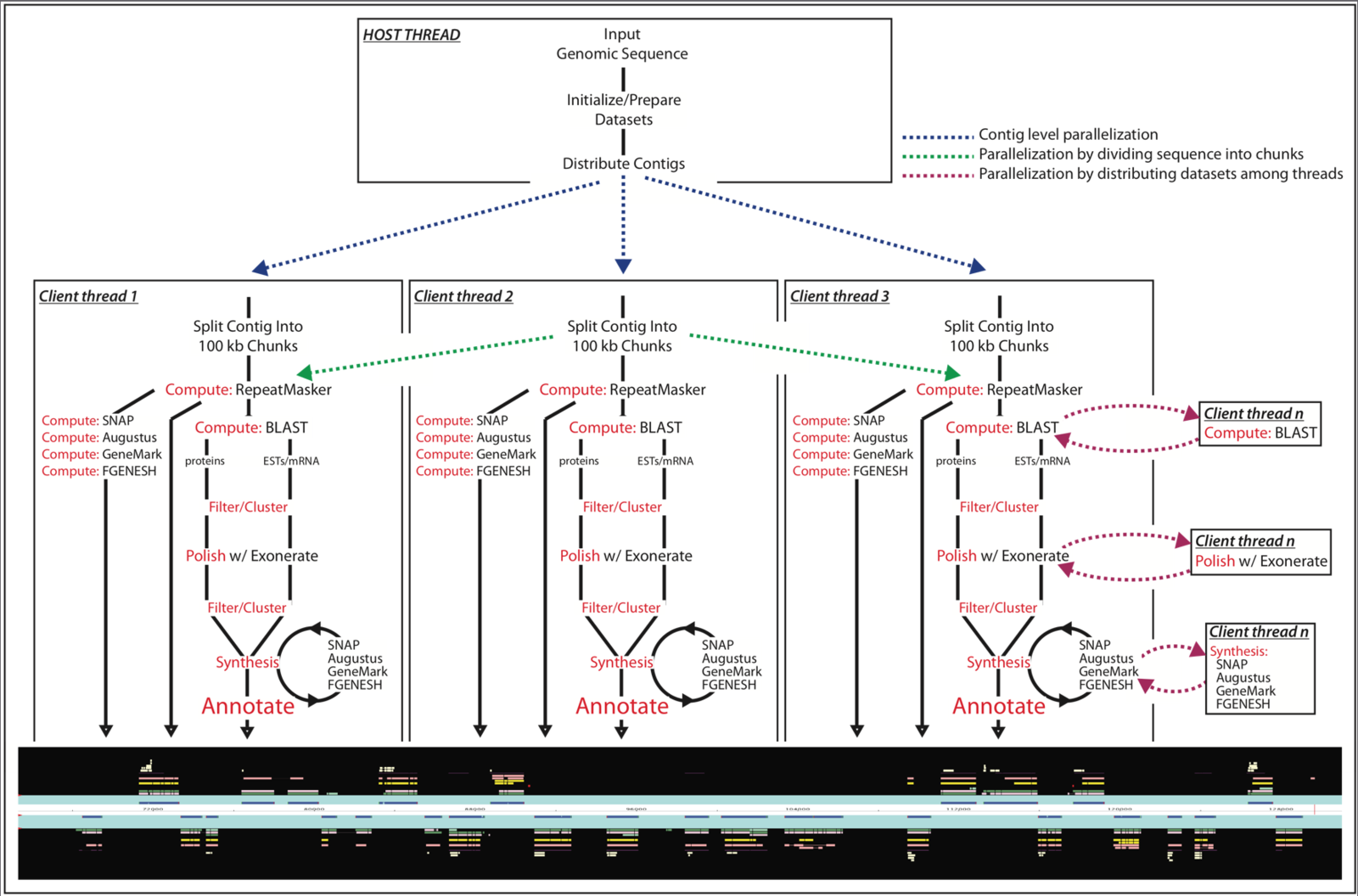
MAKER software
MAKER is a portable and easily configurable genome annotation pipeline. Its purpose is to allow smaller eukaryotic and prokaryotic genome projects to independently annotate their genomes and to create genome databases. MAKER identifies repeats, aligns ESTs and proteins to a genome, produces ab-initio gene predictions and automatically synthesizes these data into gene annotations having evidence-based quality values. MAKER is also easily trainable: outputs of preliminary runs can be used to automatically retrain its gene prediction algorithm, producing higher quality gene-models on seusequent runs. MAKER’s inputs are minimal and its ouputs can be directly loaded into a GMOD database. They can also be viewed in the Apollo genome browser; this feature of MAKER provides an easy means to annotate, view and edit individual contigs and BACs without the overhead of a database. MAKER should prove especially useful for emerging model organism projects with minimal bioinformatics expertise and computer resources.