🗺️ HPC series — you are here
1. HPC Cluster basics — SSH, file transfer, Micromamba, Slurm, dependencies 2. Resequencing pipeline on HPC — BWA-MEM2 + GATK, variant calling 3. ChIP-Seq pipeline on HPC — minimap2 + MACS3, peak calling 4. 🔵 RNA-Seq pipeline (this page) — STAR + featureCounts, DE analysis
✅ Before you start — pre-class checklist
- You can
ssh <netid>@pronghorn.rc.unr.eduand see the Pronghorn promptsacctmgr show user $USER withassocshows accountcpu-s5-bch709-6/ partitioncpu-core-0~/scratchsymlink exists and points under/data/gpfs/assoc/bch709-6/<netid>micromamba --versionworks on the login node (shell hook in~/.bashrc)- You ran the laptop version of RNA-Seq tutorial at least once so the biology makes sense
Any box unchecked? → go back to the HPC Cluster lesson first.
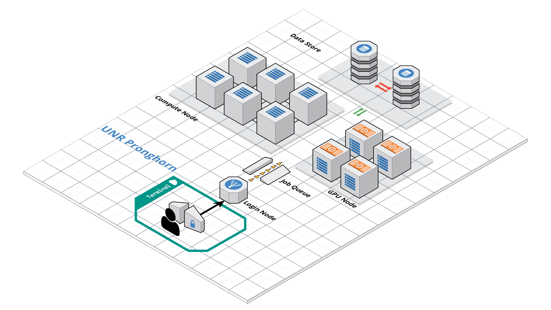
Using Pronghorn (High-Performance Computing)
Pronghorn is the University of Nevada, Reno’s new High-Performance Computing (HPC) cluster. The GPU-accelerated system is designed, built and maintained by the Office of Information Technology’s HPC Team. Pronghorn and the HPC Team supports general research across the Nevada System of Higher Education (NSHE).
Pronghorn is composed of CPU, GPU, and Storage subsystems interconnected by a 100Gb/s non-blocking Intel Omni-Path fabric. The CPU partition features 93 nodes, 2,976 CPU cores, and 21TiB of memory. The GPU partition features 44 NVIDIA Tesla P100 GPUs, 352 CPU cores, and 2.75TiB of memory. The storage system uses the IBM SpectrumScale file system to provide 1PB of high-performance storage. The computational and storage capabilities of Pronghorn will regularly expand to meet NSHE computing demands.
Pronghorn is collocated at the Switch Citadel Campus located 25 miles East of the University of Nevada, Reno. Switch is the definitive leader of sustainable data center design and operation. The Switch Citadel is rated Tier 5 Platinum, and will be the largest, most advanced data center campus on the planet.
Slurm Start Tutorial
Resource sharing on a supercomputer dedicated to technical and/or scientific computing is often organized by a piece of software called a resource manager or job scheduler. Users submit jobs, which are scheduled and allocated resources (CPU time, memory, etc.) by the resource manager.
Slurm is a resource manager and job scheduler designed to do just that, and much more. It was originally created by people at the Livermore Computing Center, and has grown into a full-fledge open-source software backed up by a large community, commercially supported by the original developers, and installed in many of the Top500 supercomputers.
Gathering information Slurm offers many commands you can use to interact with the system. For instance, the sinfo command gives an overview of the resources offered by the cluster, while the squeue command shows to which jobs those resources are currently allocated.
By default, sinfo lists the partitions that are available. A partition is a set of compute nodes (computers dedicated to… computing) grouped logically. Typical examples include partitions dedicated to batch processing, debugging, post processing, or visualization.
sinfo
sinfo
PARTITION      AVAIL  TIMELIMIT  NODES  STATE NODELIST
cpu-s2-core-0     up 14-00:00:0      2    mix cpu-[8-9]
cpu-s2-core-0     up 14-00:00:0      7  alloc cpu-[1-2,4-6,78-79]
cpu-s2-core-0     up 14-00:00:0     44   idle cpu-[0,3,7,10-47,64,76-77]
cpu-s3-core-0*    up    2:00:00      2    mix cpu-[8-9]
cpu-s3-core-0*    up    2:00:00      7  alloc cpu-[1-2,4-6,78-79]
cpu-s3-core-0*    up    2:00:00     44   idle cpu-[0,3,7,10-47,64,76-77]
gpu-s2-core-0     up 14-00:00:0     11   idle gpu-[0-10]
cpu-s6-core-0     up      15:00      2   idle cpu-[65-66]
cpu-s1-pgl-0      up 14-00:00:0      1    mix cpu-49
cpu-s1-pgl-0      up 14-00:00:0      1  alloc cpu-48
cpu-s1-pgl-0      up 14-00:00:0      2   idle cpu-[50-51]
In the above example, we see two partitions, named batch and debug. The latter is the default partition as it is marked with an asterisk. All nodes of the debug partition are idle, while two of the batch partition are being used.
The sinfo command also lists the time limit (column TIMELIMIT) to which jobs are subject. On every cluster, jobs are limited to a maximum run time, to allow job rotation and let every user a chance to see their job being started. Generally, the larger the cluster, the smaller the maximum allowed time. You can find the details on the cluster page.
You can actually specify precisely what information you would like sinfo to output by using its –format argument. For more details, have a look at the command manpage with man sinfo.
squeue
The squeue command shows the list of jobs which are currently running (they are in the RUNNING state, noted as ‘R’) or waiting for resources (noted as ‘PD’, short for PENDING).
squeue
             JOBID PARTITION     NAME     USER ST       TIME  NODES NODELIST(REASON)
            983204 cpu-s2-co    neb_K jzhang23  R 6-09:05:47      1 cpu-6
            983660 cpu-s2-co   RT3.sl yinghanc  R   12:56:17      1 cpu-9
            983659 cpu-s2-co   RT4.sl yinghanc  R   12:56:21      1 cpu-8
            983068 cpu-s2-co Gd-bound   dcantu  R 7-06:16:01      2 cpu-[78-79]
            983067 cpu-s2-co Gd-unbou   dcantu  R 1-17:41:56      2 cpu-[1-2]
            983472 cpu-s2-co   ub-all   dcantu  R 3-10:05:01      2 cpu-[4-5]
            982604 cpu-s1-pg     wrap     wyim  R 12-14:35:23      1 cpu-49
            983585 cpu-s1-pg     wrap     wyim  R 1-06:28:29      1 cpu-48
            983628 cpu-s1-pg     wrap     wyim  R   13:44:46      1 cpu-49
Text editor
SBATCH
Now the question is: How do you create a job?
A job consists in two parts: resource requests and job steps. Resource requests consist in a number of CPUs, computing expected duration, amounts of RAM or disk space, etc. Job steps describe tasks that must be done, software which must be run.
The typical way of creating a job is to write a submission script. A submission script is a shell script, e.g. a Bash script, whose comments, if they are prefixed with SBATCH, are understood by Slurm as parameters describing resource requests and other submissions options. You can get the complete list of parameters from the sbatch manpage man sbatch.
Important
The SBATCH directives must appear at the top of the submission file, before any other line except for the very first line which should be the shebang (e.g. #!/bin/bash). The script itself is a job step. Other job steps are created with the srun command. For instance, the following script, hypothetically named submit.sh,
nano submit.sh
#!/bin/bash
#SBATCH --job-name=test
#SBATCH --mail-type=all
#SBATCH --mail-user=<YOUR_EMAIL>
#SBATCH --ntasks=1
#SBATCH --mem-per-cpu=1g
#SBATCH --time=8:10:00
#SBATCH --account=cpu-s5-bch709-6
#SBATCH --partition=cpu-core-0
#SBATCH -o test_%j.out

for i in {1..1000};
do
    echo $i;
    sleep 1;
done
would request one CPU for 10 minutes, along with 1g of RAM, in the default queue. When started, the job would run a first job step srun hostname, which will launch the UNIX command hostname on the node on which the requested CPU was allocated. Then, a second job step will start the sleep command. Note that the –job-name parameter allows giving a meaningful name to the job and the –output parameter defines the file to which the output of the job must be sent.
Once the submission script is written properly, you need to submit it to slurm through the sbatch command, which, upon success, responds with the jobid attributed to the job. (The dollar sign below is the shell prompt)
chmod 775 submit.sh
sbatch submit.sh
sbatch: Submitted batch job 99999999
How to cancel the job?
scancel <JOB ID>
Scratch disk space — already set up
You already created ~/scratch (symlink to /data/gpfs/assoc/bch709-6/<your_netid>) in the HPC Cluster lesson. All paths in this lesson use ~/scratch directly. If ls -la ~/scratch doesn’t show a symlink to your scratch directory, go back and create it first.
Importing Data from the NCBI Sequence Read Archive (SRA) using the DE
Working path
cd ~/scratch
pwd
Micromamba environment
We use Micromamba for package management on Pronghorn — see the HPC Cluster lesson for installation.
micromamba create -n RNASEQ_bch709 -c conda-forge -c bioconda python=3.11 -y
micromamba activate RNASEQ_bch709

micromamba install -c conda-forge -c bioconda \
    minimap2 star 'samtools>=1.20' subread \
    openjdk=17 'trinity>=2.15' gffread seqkit kraken2 'fastp>=0.24' \
    perl-dbi perl-dbd-sqlite perl-html-parser \
    pandas numpy -y
# NOTE 1: `perl-bioperl` is intentionally NOT installed. Its current bioconda
# build pins libzlib<1.3, which conflicts with modern samtools/Trinity/kraken2.
# Trinity assembly itself does not need BioPerl — it is only required by a
# few legacy auxiliary scripts. If you ever need BioPerl, install it later
# in a SEPARATE env: `micromamba create -n bioperl -c bioconda perl-bioperl`
# NOTE 2: we deliberately do NOT install `sra-tools`. Bioconda's sra-tools 3.x
# is built against GLIBC 2.27+, newer than Pronghorn's system libc — so
# `prefetch` / `fastq-dump` crash on the compute nodes with
# "GLIBC_2.27 not found". The download steps below pull FASTQ from ENA over
# HTTPS with `curl`, which works regardless of the system GLIBC.

# Upgrade pip first — older pip can't find the prebuilt `tiktoken`
# manylinux wheel (a transitive multiqc dep), tries to build it from
# Rust source, fails on Pronghorn (no Rust compiler).
pip install --upgrade pip

# MultiQC + pinned deps. `tiktoken<0.8` is the safety pin — older
# tiktoken has stable cp311 linux wheels.
pip install --prefer-binary \
    'numpy<2.0' 'pyarrow<17' 'tiktoken<0.8' 'multiqc<1.34'
MultiQC version (read this if
multiqc.shever fails withrich.panel AttributeErrororRSEM int('#')ValueError)MultiQC 1.34 (released 2026) has two crash bugs in its module loader. The recipe above pins
'multiqc<1.34', so a fresh env is fine. Existing envs built earlier may still have 1.34 — patch with the verify→install→re-verify pattern (micromamba installfirst; fall back topiponly if the conda solver refuses to downgrade):# Step 1 — verify current micromamba run -n RNASEQ_bch709 multiqc --version # Step 2 — preferred: conda-side install (overrides any pip-installed copy) micromamba install -n RNASEQ_bch709 -c bioconda 'multiqc<1.34' -y # Step 3 — re-verify. If still 1.34, the solver kept the old version # (soft-pin from another package). Force it with pip: micromamba run -n RNASEQ_bch709 multiqc --version micromamba run -n RNASEQ_bch709 pip install -U --force-reinstall 'multiqc<1.34' # Step 4 — final verify; should print 1.33.x or earlier. micromamba run -n RNASEQ_bch709 multiqc --version
Patch libcrypto so samtools runs (do this now, not after it crashes):
Bioconda’s samtools is linked against libcrypto.so.1.0.0, but the current OpenSSL package in the env ships libcrypto.so.3 (or .1.1). Without a symlink you get:
samtools: error while loading shared libraries: libcrypto.so.1.0.0: cannot open shared object file
Create the symlink once, right after activating:
# Env must be ACTIVE so $CONDA_PREFIX points at the env folder
cd "$CONDA_PREFIX/lib"
if   [ -f libcrypto.so.1.1 ]; then ln -sf libcrypto.so.1.1 libcrypto.so.1.0.0
elif [ -f libcrypto.so.3   ]; then ln -sf libcrypto.so.3   libcrypto.so.1.0.0
fi
cd - > /dev/null

# Verify
samtools --version | head -1     # → samtools 1.xx (no libcrypto error)
If samtools --version prints a version, you’re done. If it still errors, ask the instructor before moving on.
SRA
Sequence Read Archive (SRA) data, available through multiple cloud providers and NCBI servers, is the largest publicly available repository of high throughput sequencing data. The archive accepts data from all branches of life as well as metagenomic and environmental surveys.
Searching the SRA: Searching the SRA can be complicated. Often a paper or reference will specify the accession number(s) connected to a dataset. You can search flexibly using a number of terms (such as the organism name) or the filters (e.g. DNA vs. RNA). The SRA Help Manual provides several useful explanations. It is important to know is that projects are organized and related at several levels, and some important terms include:
Bioproject: A BioProject is a collection of biological data related to a single initiative, originating from a single organization or from a consortium of coordinating organizations; see for example Bio Project 272719 Bio Sample: A description of the source materials for a project Run: These are the actual sequencing runs (usually starting with SRR); see for example SRR1761506
Publication (Arabidopsis)
SRA Bioproject site
https://www.ncbi.nlm.nih.gov/bioproject/PRJNA272719
Runinfo
| Run | ReleaseDate | LoadDate | spots | bases | spots_with_mates | avgLength | size_MB | AssemblyName | download_path | Experiment | LibraryName | LibraryStrategy | LibrarySelection | LibrarySource | LibraryLayout | InsertSize | InsertDev | Platform | Model | SRAStudy | BioProject | Study_Pubmed_id | ProjectID | Sample | BioSample | SampleType | TaxID | ScientificName | SampleName | g1k_pop_code | source | g1k_analysis_group | Subject_ID | Sex | Disease | Tumor | Affection_Status | Analyte_Type | Histological_Type | Body_Site | CenterName | Submission | dbgap_study_accession | Consent | RunHash | ReadHash |
|---|---|---|---|---|---|---|---|---|---|---|---|---|---|---|---|---|---|---|---|---|---|---|---|---|---|---|---|---|---|---|---|---|---|---|---|---|---|---|---|---|---|---|---|---|---|---|
| SRR1761506 | 1/15/2016 15:51 | 1/15/2015 12:43 | 7379945 | 1490748890 | 7379945 | 202 | 899 | https://sra-downloadb.be-md.ncbi.nlm.nih.gov/sos1/sra-pub-run-5/SRR1761506/SRR1761506.1 | SRX844600 | RNA-Seq | cDNA | TRANSCRIPTOMIC | PAIRED | 0 | 0 | ILLUMINA | Illumina HiSeq 2500 | SRP052302 | PRJNA272719 | 3 | 272719 | SRS820503 | SAMN03285048 | simple | 3702 | Arabidopsis thaliana | GSM1585887 | no | GEO | SRA232612 | public | F335FB96DDD730AC6D3AE4F6683BF234 | 12818EB5275BCB7BCB815E147BFD0619 | |||||||||||||
| SRR1761507 | 1/15/2016 15:51 | 1/15/2015 12:43 | 9182965 | 1854958930 | 9182965 | 202 | 1123 | https://sra-downloadb.be-md.ncbi.nlm.nih.gov/sos1/sra-pub-run-5/SRR1761507/SRR1761507.1 | SRX844601 | RNA-Seq | cDNA | TRANSCRIPTOMIC | PAIRED | 0 | 0 | ILLUMINA | Illumina HiSeq 2500 | SRP052302 | PRJNA272719 | 3 | 272719 | SRS820504 | SAMN03285045 | simple | 3702 | Arabidopsis thaliana | GSM1585888 | no | GEO | SRA232612 | public | 00FD62759BF7BBAEF123BF5960B2A616 | A61DCD3B96AB0796AB5E969F24F81B76 | |||||||||||||
| SRR1761508 | 1/15/2016 15:51 | 1/15/2015 12:47 | 19060611 | 3850243422 | 19060611 | 202 | 2324 | https://sra-downloadb.be-md.ncbi.nlm.nih.gov/sos1/sra-pub-run-5/SRR1761508/SRR1761508.1 | SRX844602 | RNA-Seq | cDNA | TRANSCRIPTOMIC | PAIRED | 0 | 0 | ILLUMINA | Illumina HiSeq 2500 | SRP052302 | PRJNA272719 | 3 | 272719 | SRS820505 | SAMN03285046 | simple | 3702 | Arabidopsis thaliana | GSM1585889 | no | GEO | SRA232612 | public | B75A3E64E88B1900102264522D2281CB | 657987ABC8043768E99BD82947608CAC | |||||||||||||
| SRR1761509 | 1/15/2016 15:51 | 1/15/2015 12:51 | 16555739 | 3344259278 | 16555739 | 202 | 2016 | https://sra-downloadb.be-md.ncbi.nlm.nih.gov/sos1/sra-pub-run-5/SRR1761509/SRR1761509.1 | SRX844603 | RNA-Seq | cDNA | TRANSCRIPTOMIC | PAIRED | 0 | 0 | ILLUMINA | Illumina HiSeq 2500 | SRP052302 | PRJNA272719 | 3 | 272719 | SRS820506 | SAMN03285049 | simple | 3702 | Arabidopsis thaliana | GSM1585890 | no | GEO | SRA232612 | public | 27CA2B82B69EEF56EAF53D3F464EEB7B | 2B56CA09F3655F4BBB412FD2EE8D956C | |||||||||||||
| SRR1761510 | 1/15/2016 15:51 | 1/15/2015 12:46 | 12700942 | 2565590284 | 12700942 | 202 | 1552 | https://sra-downloadb.be-md.ncbi.nlm.nih.gov/sos1/sra-pub-run-5/SRR1761510/SRR1761510.1 | SRX844604 | RNA-Seq | cDNA | TRANSCRIPTOMIC | PAIRED | 0 | 0 | ILLUMINA | Illumina HiSeq 2500 | SRP052302 | PRJNA272719 | 3 | 272719 | SRS820508 | SAMN03285050 | simple | 3702 | Arabidopsis thaliana | GSM1585891 | no | GEO | SRA232612 | public | D3901795C7ED74B8850480132F4688DA | 476A9484DCFCF9FFFDAADAAF4CE5D0EA | |||||||||||||
| SRR1761511 | 1/15/2016 15:51 | 1/15/2015 12:44 | 13353992 | 2697506384 | 13353992 | 202 | 1639 | https://sra-downloadb.be-md.ncbi.nlm.nih.gov/sos1/sra-pub-run-5/SRR1761511/SRR1761511.1 | SRX844605 | RNA-Seq | cDNA | TRANSCRIPTOMIC | PAIRED | 0 | 0 | ILLUMINA | Illumina HiSeq 2500 | SRP052302 | PRJNA272719 | 3 | 272719 | SRS820507 | SAMN03285047 | simple | 3702 | Arabidopsis thaliana | GSM1585892 | no | GEO | SRA232612 | public | 5078379601081319FCBF67C7465C404A | E3B4195AFEA115ACDA6DEF6E4AA7D8DF | |||||||||||||
| SRR1761512 | 1/15/2016 15:51 | 1/15/2015 12:44 | 8134575 | 1643184150 | 8134575 | 202 | 1067 | https://sra-downloadb.be-md.ncbi.nlm.nih.gov/sos1/sra-pub-run-5/SRR1761512/SRR1761512.1 | SRX844606 | RNA-Seq | cDNA | TRANSCRIPTOMIC | PAIRED | 0 | 0 | ILLUMINA | Illumina HiSeq 2500 | SRP052302 | PRJNA272719 | 3 | 272719 | SRS820509 | SAMN03285051 | simple | 3702 | Arabidopsis thaliana | GSM1585893 | no | GEO | SRA232612 | public | DDB8F763B71B1E29CC9C1F4C53D88D07 | 8F31604D3A4120A50B2E49329A786FA6 | |||||||||||||
| SRR1761513 | 1/15/2016 15:51 | 1/15/2015 12:43 | 7333641 | 1481395482 | 7333641 | 202 | 960 | https://sra-downloadb.be-md.ncbi.nlm.nih.gov/sos1/sra-pub-run-5/SRR1761513/SRR1761513.1 | SRX844607 | RNA-Seq | cDNA | TRANSCRIPTOMIC | PAIRED | 0 | 0 | ILLUMINA | Illumina HiSeq 2500 | SRP052302 | PRJNA272719 | 3 | 272719 | SRS820510 | SAMN03285053 | simple | 3702 | Arabidopsis thaliana | GSM1585894 | no | GEO | SRA232612 | public | 4068AE245EB0A81DFF02889D35864AF2 | 8E05C4BC316FBDFEBAA3099C54E7517B | |||||||||||||
| SRR1761514 | 1/15/2016 15:51 | 1/15/2015 12:44 | 6160111 | 1244342422 | 6160111 | 202 | 807 | https://sra-downloadb.be-md.ncbi.nlm.nih.gov/sos1/sra-pub-run-5/SRR1761514/SRR1761514.1 | SRX844608 | RNA-Seq | cDNA | TRANSCRIPTOMIC | PAIRED | 0 | 0 | ILLUMINA | Illumina HiSeq 2500 | SRP052302 | PRJNA272719 | 3 | 272719 | SRS820511 | SAMN03285059 | simple | 3702 | Arabidopsis thaliana | GSM1585895 | no | GEO | SRA232612 | public | 0A1F3E9192E7F9F4B3758B1CE514D264 | 81BFDB94C797624B34AFFEB554CE4D98 | |||||||||||||
| SRR1761515 | 1/15/2016 15:51 | 1/15/2015 12:44 | 7988876 | 1613752952 | 7988876 | 202 | 1048 | https://sra-downloadb.be-md.ncbi.nlm.nih.gov/sos1/sra-pub-run-5/SRR1761515/SRR1761515.1 | SRX844609 | RNA-Seq | cDNA | TRANSCRIPTOMIC | PAIRED | 0 | 0 | ILLUMINA | Illumina HiSeq 2500 | SRP052302 | PRJNA272719 | 3 | 272719 | SRS820512 | SAMN03285054 | simple | 3702 | Arabidopsis thaliana | GSM1585896 | no | GEO | SRA232612 | public | 39B37A0BD484C736616C5B0A45194525 | 85B031D74DF90AD1815AA1BBBF1F12BD | |||||||||||||
| SRR1761516 | 1/15/2016 15:51 | 1/15/2015 12:44 | 8770090 | 1771558180 | 8770090 | 202 | 1152 | https://sra-downloadb.be-md.ncbi.nlm.nih.gov/sos1/sra-pub-run-5/SRR1761516/SRR1761516.1 | SRX844610 | RNA-Seq | cDNA | TRANSCRIPTOMIC | PAIRED | 0 | 0 | ILLUMINA | Illumina HiSeq 2500 | SRP052302 | PRJNA272719 | 3 | 272719 | SRS820514 | SAMN03285055 | simple | 3702 | Arabidopsis thaliana | GSM1585897 | no | GEO | SRA232612 | public | E4728DFBF0F9F04B89A5B041FA570EB3 | B96545CB9C4C3EE1C9F1E8B3D4CE9D24 | |||||||||||||
| SRR1761517 | 1/15/2016 15:51 | 1/15/2015 12:44 | 8229157 | 1662289714 | 8229157 | 202 | 1075 | https://sra-downloadb.be-md.ncbi.nlm.nih.gov/sos1/sra-pub-run-5/SRR1761517/SRR1761517.1 | SRX844611 | RNA-Seq | cDNA | TRANSCRIPTOMIC | PAIRED | 0 | 0 | ILLUMINA | Illumina HiSeq 2500 | SRP052302 | PRJNA272719 | 3 | 272719 | SRS820513 | SAMN03285058 | simple | 3702 | Arabidopsis thaliana | GSM1585898 | no | GEO | SRA232612 | public | C05BC519960B075038834458514473EB | 4EF7877FC59FF5214DBF2E2FE36D67C5 | |||||||||||||
| SRR1761518 | 1/15/2016 15:51 | 1/15/2015 12:44 | 8760931 | 1769708062 | 8760931 | 202 | 1072 | https://sra-downloadb.be-md.ncbi.nlm.nih.gov/sos1/sra-pub-run-5/SRR1761518/SRR1761518.1 | SRX844612 | RNA-Seq | cDNA | TRANSCRIPTOMIC | PAIRED | 0 | 0 | ILLUMINA | Illumina HiSeq 2500 | SRP052302 | PRJNA272719 | 3 | 272719 | SRS820515 | SAMN03285052 | simple | 3702 | Arabidopsis thaliana | GSM1585899 | no | GEO | SRA232612 | public | 7D8333182062545CECD5308A222FF506 | 382F586C4BF74E474D8F9282E36BE4EC | |||||||||||||
| SRR1761519 | 1/15/2016 15:51 | 1/15/2015 12:44 | 6643107 | 1341907614 | 6643107 | 202 | 811 | https://sra-downloadb.be-md.ncbi.nlm.nih.gov/sos1/sra-pub-run-5/SRR1761519/SRR1761519.1 | SRX844613 | RNA-Seq | cDNA | TRANSCRIPTOMIC | PAIRED | 0 | 0 | ILLUMINA | Illumina HiSeq 2500 | SRP052302 | PRJNA272719 | 3 | 272719 | SRS820516 | SAMN03285056 | simple | 3702 | Arabidopsis thaliana | GSM1585900 | no | GEO | SRA232612 | public | 163BD8073D7E128D8AD1B253A722DD08 | DFBCC891EB5FA97490E32935E54C9E14 | |||||||||||||
| SRR1761520 | 1/15/2016 15:51 | 1/15/2015 12:44 | 8506472 | 1718307344 | 8506472 | 202 | 1040 | https://sra-downloadb.be-md.ncbi.nlm.nih.gov/sos1/sra-pub-run-5/SRR1761520/SRR1761520.1 | SRX844614 | RNA-Seq | cDNA | TRANSCRIPTOMIC | PAIRED | 0 | 0 | ILLUMINA | Illumina HiSeq 2500 | SRP052302 | PRJNA272719 | 3 | 272719 | SRS820517 | SAMN03285062 | simple | 3702 | Arabidopsis thaliana | GSM1585901 | no | GEO | SRA232612 | public | 791BD0D8840AA5F1D74E396668638DA1 | AF4694425D34F84095F6CFD6F4A09936 | |||||||||||||
| SRR1761521 | 1/15/2016 15:51 | 1/15/2015 12:46 | 13166085 | 2659549170 | 13166085 | 202 | 1609 | https://sra-downloadb.be-md.ncbi.nlm.nih.gov/sos1/sra-pub-run-5/SRR1761521/SRR1761521.1 | SRX844615 | RNA-Seq | cDNA | TRANSCRIPTOMIC | PAIRED | 0 | 0 | ILLUMINA | Illumina HiSeq 2500 | SRP052302 | PRJNA272719 | 3 | 272719 | SRS820518 | SAMN03285057 | simple | 3702 | Arabidopsis thaliana | GSM1585902 | no | GEO | SRA232612 | public | 47C40480E9B7DB62B4BEE0F2193D16B3 | 1443C58A943C07D3275AB12DC31644A9 | |||||||||||||
| SRR1761522 | 1/15/2016 15:51 | 1/15/2015 12:49 | 9496483 | 1918289566 | 9496483 | 202 | 1162 | https://sra-downloadb.be-md.ncbi.nlm.nih.gov/sos1/sra-pub-run-5/SRR1761522/SRR1761522.1 | SRX844616 | RNA-Seq | cDNA | TRANSCRIPTOMIC | PAIRED | 0 | 0 | ILLUMINA | Illumina HiSeq 2500 | SRP052302 | PRJNA272719 | 3 | 272719 | SRS820519 | SAMN03285061 | simple | 3702 | Arabidopsis thaliana | GSM1585903 | no | GEO | SRA232612 | public | BB05DF11E1F95427530D69DB5E0FA667 | 7706862FB2DF957E4041D2064A691CF6 | |||||||||||||
| SRR1761523 | 1/15/2016 15:51 | 1/15/2015 12:46 | 14999315 | 3029861630 | 14999315 | 202 | 1832 | https://sra-downloadb.be-md.ncbi.nlm.nih.gov/sos1/sra-pub-run-5/SRR1761523/SRR1761523.1 | SRX844617 | RNA-Seq | cDNA | TRANSCRIPTOMIC | PAIRED | 0 | 0 | ILLUMINA | Illumina HiSeq 2500 | SRP052302 | PRJNA272719 | 3 | 272719 | SRS820520 | SAMN03285060 | simple | 3702 | Arabidopsis thaliana | GSM1585904 | no | GEO | SRA232612 | public | 101D3A151E632224C09A702BD2F59CF5 | 0AC99FAA6B8941F89FFCBB8B1910696E |
Subset of data
| Sample information | Run |
|---|---|
| WT_rep1 | SRR1761506 |
| WT_rep2 | SRR1761507 |
| WT_rep3 | SRR1761508 |
| ABA_rep1 | SRR1761509 |
| ABA_rep2 | SRR1761510 |
| ABA_rep3 | SRR1761511 |
🔁 Already ran fastq-dump + trim in HPC_cluster?
The HPC Cluster lesson Workflow Step 1·2 downloads the same Arabidopsis SRR1761506-511 dataset and trims with fastp into the shared workspace at
~/scratch/rnaseq/raw_data/and~/scratch/rnaseq/trim/. To reuse those results here (no need to re-download or re-trim):# Sanity-check the shared workspace already has the trimmed reads ls ~/scratch/rnaseq/trim/SRR1761506_1.trimmed.fq.gz \ ~/scratch/rnaseq/trim/SRR1761506_2.trimmed.fq.gz # Set up the ATH project sub-directory under the shared parent mkdir -p ~/scratch/rnaseq/ATH cd ~/scratch/rnaseq/ATH ln -s ~/scratch/rnaseq/raw_data raw_data # reuse existing FASTQ ln -s ~/scratch/rnaseq/trim trim # reuse trimmed reads mkdir -p reference bam logs # only the new directories (logs/ for Slurm stdout)If the
lsabove prints both files, skip to “Reference downloads” below — STAR index + alignment is where this lesson really starts. Otherwise (fresh start, no HPC_cluster prerequisites done), follow the standard setup below.
mkdir -p ~/scratch/rnaseq/ATH
cd ~/scratch/rnaseq/ATH
mkdir -p raw_data trim reference bam logs
pwd
FASTQ download submission (from ENA)
Bioconda’s sra-tools 3.x crashes on Pronghorn (built against GLIBC 2.27+, newer than the system libc). We pull the same FASTQ from ENA, which mirrors every SRA run as ready-to-use .fastq.gz over HTTPS — no SRA toolkit needed.
cd ~/scratch/rnaseq/ATH
nano fastq-dump.sh
#!/bin/bash
#SBATCH --job-name=fastqdump_ATH
#SBATCH --cpus-per-task=2
#SBATCH --time=2-15:00:00
#SBATCH --mem=16g
#SBATCH --mail-type=all
#SBATCH --mail-user=<YOUR_EMAIL>
#SBATCH -o fastq-dump.out # STDOUT & STDERR
#SBATCH --account=cpu-s5-bch709-6
#SBATCH --partition=cpu-core-0

set -euo pipefail
mkdir -p ./raw_data

for SRR in SRR1761506 SRR1761507 SRR1761508 SRR1761509 SRR1761510 SRR1761511; do
  URLS=$(curl -fsSL --retry 3 --max-time 60 \
          "https://www.ebi.ac.uk/ena/portal/api/filereport?accession=${SRR}&result=read_run&fields=fastq_ftp&format=tsv" \
          | tail -n +2 | awk -F'\t' '{print $NF}' | tr ';' '\n' | sed '/^$/d')
  [ -n "${URLS}" ] || { echo "ERROR: ENA returned no fastq URLs for ${SRR}"; exit 1; }
  for U in ${URLS}; do
    OUT=./raw_data/$(basename "${U}")
    # Skip-by-existence removed intentionally — a partial download (e.g. a
    # 960 MB chunk of a 1.2 GB file from a previous job that was cancelled
    # mid-stream) would silently pass `[ -s "${OUT}" ]` and corrupt the
    # rest of the pipeline. `curl -C -` below either resumes such partials
    # or exits cleanly when the file is already complete.
    echo "[fastq] ${SRR} -> https://${U}"
    # --retry-all-errors: retry on SSL eof / connection drops (EBI HTTPS
    #   regularly drops mid-stream on >1 GB transfers; without this flag,
    #   curl --retry only retries on HTTP 5xx and exits 56 on SSL eof).
    # -C -: resume partial downloads. If ${OUT} is already complete, curl
    #   detects it and exits cleanly without re-downloading.
    # --retry bumped to 5 for headroom on consecutive drops.
    curl -fsSL --retry 5 --retry-all-errors --retry-delay 30 \
         --max-time 3600 -C - -o "${OUT}" "https://${U}"
  done
done
Read Trimming with fastp
cd  ~/scratch/rnaseq/ATH
nano trim.sh
#!/bin/bash
#SBATCH --job-name=trim_ATH
#SBATCH --cpus-per-task=2
#SBATCH --time=2-15:00:00
#SBATCH --mem=16g
#SBATCH --mail-type=all
#SBATCH --mail-user=<YOUR_EMAIL>
#SBATCH -o trim.out # STDOUT & STDERR
#SBATCH --account=cpu-s5-bch709-6
#SBATCH --partition=cpu-core-0

fastp --in1 raw_data/SRR1761506_1.fastq.gz --in2 raw_data/SRR1761506_2.fastq.gz --out1 trim/SRR1761506_1.trimmed.fq.gz --out2 trim/SRR1761506_2.trimmed.fq.gz --detect_adapter_for_pe --qualified_quality_phred 20 --length_required 50 --thread 2 --html trim/SRR1761506_fastp.html --json trim/SRR1761506_fastp.json
fastp --in1 raw_data/SRR1761507_1.fastq.gz --in2 raw_data/SRR1761507_2.fastq.gz --out1 trim/SRR1761507_1.trimmed.fq.gz --out2 trim/SRR1761507_2.trimmed.fq.gz --detect_adapter_for_pe --qualified_quality_phred 20 --length_required 50 --thread 2 --html trim/SRR1761507_fastp.html --json trim/SRR1761507_fastp.json
fastp --in1 raw_data/SRR1761508_1.fastq.gz --in2 raw_data/SRR1761508_2.fastq.gz --out1 trim/SRR1761508_1.trimmed.fq.gz --out2 trim/SRR1761508_2.trimmed.fq.gz --detect_adapter_for_pe --qualified_quality_phred 20 --length_required 50 --thread 2 --html trim/SRR1761508_fastp.html --json trim/SRR1761508_fastp.json
fastp --in1 raw_data/SRR1761509_1.fastq.gz --in2 raw_data/SRR1761509_2.fastq.gz --out1 trim/SRR1761509_1.trimmed.fq.gz --out2 trim/SRR1761509_2.trimmed.fq.gz --detect_adapter_for_pe --qualified_quality_phred 20 --length_required 50 --thread 2 --html trim/SRR1761509_fastp.html --json trim/SRR1761509_fastp.json
fastp --in1 raw_data/SRR1761510_1.fastq.gz --in2 raw_data/SRR1761510_2.fastq.gz --out1 trim/SRR1761510_1.trimmed.fq.gz --out2 trim/SRR1761510_2.trimmed.fq.gz --detect_adapter_for_pe --qualified_quality_phred 20 --length_required 50 --thread 2 --html trim/SRR1761510_fastp.html --json trim/SRR1761510_fastp.json
fastp --in1 raw_data/SRR1761511_1.fastq.gz --in2 raw_data/SRR1761511_2.fastq.gz --out1 trim/SRR1761511_1.trimmed.fq.gz --out2 trim/SRR1761511_2.trimmed.fq.gz --detect_adapter_for_pe --qualified_quality_phred 20 --length_required 50 --thread 2 --html trim/SRR1761511_fastp.html --json trim/SRR1761511_fastp.json
Reference downloads
We download the Arabidopsis TAIR10 genome and annotation directly from TAIR (www.arabidopsis.org). No JGI/Phytozome account required, no zip-bundle to unpack.
cd ~/scratch/rnaseq/ATH
mkdir -p bam reference logs
cd reference
pwd
Download Arabidopsis thaliana TAIR10 from TAIR
TAIR’s API serves the canonical TAIR10 chromosome FASTA and GFF3. The host uses a self-signed certificate, so we pass -k to curl (same as wget --no-check-certificate).
cd ~/scratch/rnaseq/ATH/reference

# Genome FASTA (gzipped, ~35 MB)
curl -kfsSL --retry 3 --max-time 600 \
    -o TAIR10_chr_all.fas.gz \
    "https://www.arabidopsis.org/api/download-files/download?filePath=Genes/TAIR10_genome_release/TAIR10_chromosome_files/TAIR10_chr_all.fas.gz"
gunzip -f TAIR10_chr_all.fas.gz

# Gene annotation (GFF3)
curl -kfsSL --retry 3 --max-time 600 \
    -o TAIR10_GFF3_genes.gff \
    "https://www.arabidopsis.org/api/download-files/download?filePath=Genes/TAIR10_genome_release/TAIR10_gff3/TAIR10_GFF3_genes.gff"

ls -lh TAIR10_chr_all.fas TAIR10_GFF3_genes.gff
seqkit stats TAIR10_chr_all.fas
Convert GFF to GTF
STAR’s --sjdbGTFfile expects GTF, so we convert the GFF3 with gffread:
cd ~/scratch/rnaseq/ATH/reference
gffread TAIR10_GFF3_genes.gff -T -F --keep-exon-attrs -o TAIR10_GFF3_genes.gtf
Create reference index
cd  ~/scratch/rnaseq/ATH/reference
ls -algh
nano index.sh
#!/bin/bash
#SBATCH --job-name=index_ATH
#SBATCH --cpus-per-task=12
#SBATCH --time=2-15:00:00
#SBATCH --mem=48g
#SBATCH --mail-type=all
#SBATCH --mail-user=<YOUR_EMAIL>
#SBATCH -o index.out # STDOUT & STDERR
#SBATCH --account=cpu-s5-bch709-6
#SBATCH --partition=cpu-core-0

STAR --runThreadN 12 --runMode genomeGenerate --genomeDir . --genomeFastaFiles TAIR10_chr_all.fas --sjdbGTFfile TAIR10_GFF3_genes.gtf --sjdbOverhang 99 --genomeSAindexNbases 12
Mapping the reads to genome index
cd  ~/scratch/rnaseq/ATH/
ls -algh
nano align.sh
#!/bin/bash
#SBATCH --job-name=align_ATH
#SBATCH --cpus-per-task=8
#SBATCH --time=2-15:00:00
#SBATCH --mem=32g
#SBATCH --mail-type=all
#SBATCH --mail-user=<YOUR_EMAIL>
#SBATCH -o align.out # STDOUT & STDERR
#SBATCH --account=cpu-s5-bch709-6
#SBATCH --partition=cpu-core-0
# NOTE: do NOT hard-code --dependency here. Pass it on the `sbatch` command line
# so the job ID is filled in automatically — see the "Submit the pipeline with
# dependency chaining" section below.

STAR --runMode alignReads --runThreadN 8 --readFilesCommand zcat --outFilterMultimapNmax 10 --alignIntronMin 25 --alignIntronMax 10000 --genomeDir ~/scratch/rnaseq/ATH/reference/ --readFilesIn ~/scratch/rnaseq/ATH/trim/SRR1761506_1.trimmed.fq.gz ~/scratch/rnaseq/ATH/trim/SRR1761506_2.trimmed.fq.gz --outSAMtype BAM SortedByCoordinate --outFileNamePrefix ~/scratch/rnaseq/ATH/bam/SRR1761506.bam

STAR --runMode alignReads --runThreadN 8 --readFilesCommand zcat --outFilterMultimapNmax 10 --alignIntronMin 25 --alignIntronMax 10000 --genomeDir ~/scratch/rnaseq/ATH/reference/ --readFilesIn ~/scratch/rnaseq/ATH/trim/SRR1761507_1.trimmed.fq.gz ~/scratch/rnaseq/ATH/trim/SRR1761507_2.trimmed.fq.gz --outSAMtype BAM SortedByCoordinate --outFileNamePrefix ~/scratch/rnaseq/ATH/bam/SRR1761507.bam

STAR --runMode alignReads --runThreadN 8 --readFilesCommand zcat --outFilterMultimapNmax 10 --alignIntronMin 25 --alignIntronMax 10000 --genomeDir ~/scratch/rnaseq/ATH/reference/ --readFilesIn ~/scratch/rnaseq/ATH/trim/SRR1761508_1.trimmed.fq.gz ~/scratch/rnaseq/ATH/trim/SRR1761508_2.trimmed.fq.gz --outSAMtype BAM SortedByCoordinate --outFileNamePrefix ~/scratch/rnaseq/ATH/bam/SRR1761508.bam

STAR --runMode alignReads --runThreadN 8 --readFilesCommand zcat --outFilterMultimapNmax 10 --alignIntronMin 25 --alignIntronMax 10000 --genomeDir ~/scratch/rnaseq/ATH/reference/ --readFilesIn ~/scratch/rnaseq/ATH/trim/SRR1761509_1.trimmed.fq.gz ~/scratch/rnaseq/ATH/trim/SRR1761509_2.trimmed.fq.gz --outSAMtype BAM SortedByCoordinate --outFileNamePrefix ~/scratch/rnaseq/ATH/bam/SRR1761509.bam

STAR --runMode alignReads --runThreadN 8 --readFilesCommand zcat --outFilterMultimapNmax 10 --alignIntronMin 25 --alignIntronMax 10000 --genomeDir ~/scratch/rnaseq/ATH/reference/ --readFilesIn ~/scratch/rnaseq/ATH/trim/SRR1761510_1.trimmed.fq.gz ~/scratch/rnaseq/ATH/trim/SRR1761510_2.trimmed.fq.gz --outSAMtype BAM SortedByCoordinate --outFileNamePrefix ~/scratch/rnaseq/ATH/bam/SRR1761510.bam

STAR --runMode alignReads --runThreadN 8 --readFilesCommand zcat --outFilterMultimapNmax 10 --alignIntronMin 25 --alignIntronMax 10000 --genomeDir ~/scratch/rnaseq/ATH/reference/ --readFilesIn ~/scratch/rnaseq/ATH/trim/SRR1761511_1.trimmed.fq.gz ~/scratch/rnaseq/ATH/trim/SRR1761511_2.trimmed.fq.gz --outSAMtype BAM SortedByCoordinate --outFileNamePrefix ~/scratch/rnaseq/ATH/bam/SRR1761511.bam
Counting reads with featureCounts — featureCounts.sh
Once every BAM is sorted by coordinate, count read pairs against the TAIR10 GTF. With subread ≥ 2.0.2, paired-end fragment counting requires both -p (paired-end) and --countReadPairs (count pairs as 1 rather than 2). The output ATH.featureCount.cnt is what the MultiQC and DESeq2/EdgeR steps below consume.
cd ~/scratch/rnaseq/ATH
nano featureCounts.sh
#!/bin/bash
#SBATCH --job-name=featurecounts_ATH
#SBATCH --cpus-per-task=8
#SBATCH --time=06:00:00
#SBATCH --mem=16g
#SBATCH --mail-type=FAIL,END
#SBATCH --mail-user=<YOUR_EMAIL>
#SBATCH -o logs/featurecounts_%j.out
#SBATCH --account=cpu-s5-bch709-6
#SBATCH --partition=cpu-core-0

set -euo pipefail
PROJECT=~/scratch/rnaseq/ATH
cd "$PROJECT/bam"

# Hard-coded SRR list — matches the cohort used in fastq-dump.sh / align.sh above.
BAMS="SRR1761506.bamAligned.sortedByCoord.out.bam \
      SRR1761507.bamAligned.sortedByCoord.out.bam \
      SRR1761508.bamAligned.sortedByCoord.out.bam \
      SRR1761509.bamAligned.sortedByCoord.out.bam \
      SRR1761510.bamAligned.sortedByCoord.out.bam \
      SRR1761511.bamAligned.sortedByCoord.out.bam"

featureCounts \
    -T 8 \
    -p --countReadPairs \
    -a "$PROJECT/reference/TAIR10_GFF3_genes.gtf" \
    -o ATH.featureCount.cnt \
    ${BAMS}
Submit & inspect (standalone):
sbatch featureCounts.sh
# when done:
cat ~/scratch/rnaseq/ATH/bam/ATH.featureCount.cnt.summary
(run_all.sh below wires this in automatically — you don’t need to submit it by hand.)
Submit the entire pipeline with one script — run_all.sh
Rather than running each step by hand (submit → wait → submit → wait…), put every step into a driver script that submits them all at once. Slurm queues each job in the right order using --dependency; the whole pipeline runs unattended.
Pipeline DAG:
  fastq-dump ──┐
               ├─→ trim ─→ align ─→ featureCounts ─→ multiqc
  index   ─────┘
(Download + index run in parallel; trim waits on download; align waits on both trim and index; featureCounts waits on align; multiqc waits on featureCounts.)
Save as run_all.sh:
#!/bin/bash
# run_all.sh — submit the entire Arabidopsis RNA-Seq pipeline with one command.
# Slurm enforces the correct order via --dependency; you can walk away.
set -euo pipefail

PROJECT=~/scratch/rnaseq/ATH
cd "$PROJECT"

# Activate the env in THIS shell so every sbatch below inherits the PATH
# (sbatch --export=ALL is the default — the submitted jobs see the same tools)
export MAMBA_ROOT_PREFIX="${MAMBA_ROOT_PREFIX:-$HOME/micromamba}"
eval "$(micromamba shell hook --shell=bash)"
micromamba activate RNASEQ_bch709

# 1. Download FASTQs (no prerequisites)
DUMP_JID=$(sbatch --parsable fastq-dump.sh)

# 2. Build STAR index (independent of download — runs in parallel)
IDX_JID=$(cd "$PROJECT/reference" && sbatch --parsable index.sh)

# 3. Trim reads (waits for download)
TRIM_JID=$(sbatch --parsable --dependency=afterok:${DUMP_JID} trim.sh)

# 4. Align to genome (waits for BOTH trim and index)
ALIGN_JID=$(sbatch --parsable --dependency=afterok:${TRIM_JID}:${IDX_JID} align.sh)

# 5. featureCounts (waits for align)
FC_JID=$(sbatch --parsable --dependency=afterok:${ALIGN_JID} featureCounts.sh)

# 6. MultiQC aggregation (waits for featureCounts; afterany lets it run even if FC partially failed)
MQC_JID=$(sbatch --parsable --dependency=afterany:${FC_JID} multiqc.sh)

cat <<EOF
Submitted RNA-Seq pipeline (Arabidopsis):
  fastq-dump      ${DUMP_JID}
  index           ${IDX_JID}
  trim            ${TRIM_JID}
  align           ${ALIGN_JID}
  featureCounts   ${FC_JID}
  multiqc         ${MQC_JID}

Monitor with:  squeue -u \$USER
Cancel all:    scancel ${DUMP_JID} ${IDX_JID} ${TRIM_JID} ${ALIGN_JID} ${FC_JID} ${MQC_JID}
Final report (after pipeline finishes): ~/scratch/rnaseq/ATH/qc/ATH_report.html
EOF
Run it:
chmod +x run_all.sh
bash run_all.sh
squeue -u $USER   # later jobs show state PD with reason (Dependency)
You’ll see 4 job IDs printed immediately. Close your laptop — Slurm takes over. When everything finishes, check ls bam/ for sorted BAM outputs and log files for Finished successfully.
🧑💻 Hands-on walkthrough — submit the pipeline step-by-step
If you want to see exactly what run_all.sh does (or debug one step), submit each stage manually. Every sbatch returns a job ID that the next step depends on.
Do this first (login shell — one time):
micromamba activate RNASEQ_bch709
cd ~/scratch/rnaseq/ATH
Then submit each step — each line is one command:
# --- Step 1: download FASTQs (no prerequisites) ---
DUMP_JID=$(sbatch --parsable fastq-dump.sh)
echo "fastq-dump → $DUMP_JID"

# --- Step 2: build STAR index (no prerequisites, runs in parallel with Step 1) ---
IDX_JID=$(cd reference && sbatch --parsable index.sh)
echo "index      → $IDX_JID"

# --- Step 3: trim (waits for fastq-dump) ---
TRIM_JID=$(sbatch --parsable --dependency=afterok:${DUMP_JID} trim.sh)
echo "trim       → $TRIM_JID"

# --- Step 4: align (waits for BOTH trim and index) ---
ALIGN_JID=$(sbatch --parsable --dependency=afterok:${TRIM_JID}:${IDX_JID} align.sh)
echo "align      → $ALIGN_JID"

# --- Step 5: featureCounts (waits for align) ---
FC_JID=$(sbatch --parsable --dependency=afterok:${ALIGN_JID} featureCounts.sh)
echo "featureCounts → $FC_JID"

# --- Step 6: MultiQC (waits for featureCounts) ---
MQC_JID=$(sbatch --parsable --dependency=afterany:${FC_JID} multiqc.sh)
echo "multiqc    → $MQC_JID"

# Check that everything is queued
squeue -u $USER
# Steps 3-6 should show state PD with reason (Dependency)
Why copy the commands into your terminal, not a script?
The hands-on walkthrough is literally what
run_all.shdoes — but by typing each line you see each job ID appear and can inspect things in between. Once you’re comfortable, just runbash run_all.shnext time.
Same pattern for every other organism
For Drosophila, Mouse, Tomato, Mosquito, etc., copy
run_all.shinto that organism’s project directory, updatePROJECT=~/scratch/rnaseq/<ORG>, and run it. The script structure doesn’t change — only the path.
Don’t hard-code dependencies inside the
#SBATCHblockSome older examples had
#SBATCH --dependency=afterok:<PREVIOUS_JOBID(trim_ATH)>insidealign.sh. That’s fragile — you’d have to edit the file and paste the previous job’s ID every single time. Instead, pass--dependencyon thesbatchcommand line (as shown inrun_all.shabove). If you see a#SBATCH --dependency=...line inside any script, delete it.
For a full explanation of --dependency, afterok vs afterany, and the --parsable flag, see the Job dependencies section in the HPC Cluster lesson.
micromamba install -c conda-forge tree
Drosophila
Publication (Drosophila)
Not formally published — data deposited at NCBI as PRJNA770108 (Gene expression profiling of D. melanogaster larval brains after chronic alcohol exposure).
✅ Before you start the Drosophila walkthrough — pre-class checklist
- You finished the Arabidopsis section above (or at least understand
sbatch,--dependency, andrun_all.sh)micromamba activate RNASEQ_bch709works in your login shell (STAR, fastp, subread/featureCounts, multiqc all on PATH)~/scratch/rnaseq/already exists from the Arabidopsis run; we’ll addDrosophila/next toATH/- You have ~8 GB free under
~/scratch(6 PE samples × ~30 M reads + STAR index + BAMs)- You replaced
<YOUR_EMAIL>in your previous SBATCH headers — keep doing that hereAny box unchecked? → re-read the Arabidopsis run_all.sh walkthrough before continuing.
🪰 Drosophila-specific notes (vs. Arabidopsis)
- Longer introns →
--alignIntronMax 100000(Arabidopsis used 10 000). The longest D. melanogaster introns reach ~70 kb.- Smaller genome (~143 Mb) →
--genomeSAindexNbases 12(same value used for ATH; smaller-than-default 14 keeps the SA index in-RAM)- Cohort: 6 paired-end samples (~25–35 M read pairs each), 3 ethanol-treated vs 3 controls — perfect for a 2-group DESeq2 contrast
- Reference: FlyBase r6.42 (FB2021_05). Genome FASTA + GTF come straight from
ftp.flybase.net; Ensembl BDGP6.32 r104 is kept as a fallback mirror infastq-dump.shstyle.
SRA Bioproject site
https://www.ncbi.nlm.nih.gov/bioproject/PRJNA770108
Gene expression profiling of Drosophila melanogaster larval brains after chronic alcohol exposure (fruit fly)
We sequenced mRNA extracted from brains of (1) D. melanogaster larvae exposed to food containing 5% ethanol (v/v) for 6 consecutive days, and (2) age-matched untreated control larvae that grew in regular food. Differential gene expression between the two groups was calculated and reported. Each group consisted of 3 biological replicates of 30 brains each. Overall design: examination of mRNA levels in brains of D. melanogaster larvae after chronic ethanol exposure was performed using next generation sequencing (RNA-seq).
Subset of data
| Sample information | Run |
|---|---|
| Control | SRR16287545 |
| Control | SRR16287546 |
| Control | SRR16287547 |
| Ethanol treatment | SRR16287548 |
| Ethanol treatment | SRR16287549 |
| Ethanol treatment | SRR16287550 |
Project layout
mkdir -p ~/scratch/rnaseq
cd ~/scratch/rnaseq
mkdir -p Drosophila && cd Drosophila
mkdir -p raw_data trim bam reference logs qc
pwd
# example output (your <netid> will differ)
/data/gpfs/assoc/bch709-6/<netid>/scratch/rnaseq/Drosophila
samples.txt — one place to list the cohort
Every script below reads samples.txt so you only edit the cohort once. Tab-delimited: sample_name<TAB>SRR<TAB>condition. The header row exists so the awk loops can simply NR>1 to skip it.
cd ~/scratch/rnaseq/Drosophila
nano samples.txt
Paste exactly (real tab characters between columns — nano writes them literally):
sample	srr	condition
ctrl_rep1	SRR16287545	Control
ctrl_rep2	SRR16287546	Control
ctrl_rep3	SRR16287547	Control
etoh_rep1	SRR16287548	Ethanol
etoh_rep2	SRR16287549	Ethanol
etoh_rep3	SRR16287550	Ethanol
Verify:
cat samples.txt
awk -F'\t' 'NR>1{print $2}' samples.txt   # SRR list the loops will iterate over
sample	srr	condition
ctrl_rep1	SRR16287545	Control
ctrl_rep2	SRR16287546	Control
ctrl_rep3	SRR16287547	Control
etoh_rep1	SRR16287548	Ethanol
etoh_rep2	SRR16287549	Ethanol
etoh_rep3	SRR16287550	Ethanol

SRR16287545
SRR16287546
SRR16287547
SRR16287548
SRR16287549
SRR16287550
fastq download (from ENA)
Same ENA-over-HTTPS approach as Arabidopsis (no broken sra-tools GLIBC dependency). The loop reads SRR IDs from samples.txt instead of being hard-coded.
cd ~/scratch/rnaseq/Drosophila
nano fastq-dump.sh
#!/bin/bash
#SBATCH --job-name=fastqdump_Drosophila
#SBATCH --cpus-per-task=2
#SBATCH --time=2-15:00:00
#SBATCH --mem=16g
#SBATCH --mail-type=all
#SBATCH --mail-user=<YOUR_EMAIL>
#SBATCH -o logs/fastq-dump_%j.out  # STDOUT & STDERR
#SBATCH --account=cpu-s5-bch709-6
#SBATCH --partition=cpu-core-0

set -euo pipefail
PROJECT=~/scratch/rnaseq/Drosophila
cd "$PROJECT"
mkdir -p raw_data logs

# Drive the loop from samples.txt (column 2 = SRR; NR>1 skips the header)
SRRS=$(awk -F'\t' 'NR>1{print $2}' samples.txt)

for SRR in ${SRRS}; do
  URLS=$(curl -fsSL --retry 3 --max-time 60 \
          "https://www.ebi.ac.uk/ena/portal/api/filereport?accession=${SRR}&result=read_run&fields=fastq_ftp&format=tsv" \
          | tail -n +2 | awk -F'\t' '{print $NF}' | tr ';' '\n' | sed '/^$/d')
  [ -n "${URLS}" ] || { echo "ERROR: ENA returned no fastq URLs for ${SRR}"; exit 1; }
  for U in ${URLS}; do
    OUT=raw_data/$(basename "${U}")
    # Skip-by-existence removed intentionally — a partial download (e.g. a
    # 960 MB chunk of a 1.2 GB file from a previous job that was cancelled
    # mid-stream) would silently pass `[ -s "${OUT}" ]` and corrupt the
    # rest of the pipeline. `curl -C -` below either resumes such partials
    # or exits cleanly when the file is already complete.
    echo "[fastq] ${SRR} -> https://${U}"
    # --retry-all-errors: retry on SSL eof / connection drops (EBI HTTPS
    #   regularly drops mid-stream on >1 GB transfers; without this flag,
    #   curl --retry only retries on HTTP 5xx and exits 56 on SSL eof).
    # -C -: resume partial downloads. If ${OUT} is already complete, curl
    #   detects it and exits cleanly without re-downloading.
    # --retry bumped to 5 for headroom on consecutive drops.
    curl -fsSL --retry 5 --retry-all-errors --retry-delay 30 \
         --max-time 3600 -C - -o "${OUT}" "https://${U}"
  done
done

ls -lh raw_data/*.fastq.gz
Submit & inspect:
sbatch fastq-dump.sh
# wait for completion, then (full paths so this works regardless of cwd):
tail -n 20 ~/scratch/rnaseq/Drosophila/logs/fastq-dump_<jobid>.out
ls -lh    ~/scratch/rnaseq/Drosophila/raw_data/
# example tail (your numbers will differ)
[fastq] SRR16287545 -> https://ftp.sra.ebi.ac.uk/vol1/fastq/SRR162/045/SRR16287545/SRR16287545_1.fastq.gz
[fastq] SRR16287545 -> https://ftp.sra.ebi.ac.uk/vol1/fastq/SRR162/045/SRR16287545/SRR16287545_2.fastq.gz
[fastq] SRR16287546 -> https://ftp.sra.ebi.ac.uk/vol1/fastq/SRR162/046/SRR16287546/SRR16287546_1.fastq.gz
...
[fastq] SRR16287550 -> https://ftp.sra.ebi.ac.uk/vol1/fastq/SRR162/050/SRR16287550/SRR16287550_2.fastq.gz
-rw-r--r-- 1 <netid> users 1.6G ... raw_data/SRR16287545_1.fastq.gz
-rw-r--r-- 1 <netid> users 1.7G ... raw_data/SRR16287545_2.fastq.gz
-rw-r--r-- 1 <netid> users 1.5G ... raw_data/SRR16287550_2.fastq.gz
Read trimming with fastp — loop driven by samples.txt
Instead of 6 hard-coded fastp lines, loop over the SRR column of samples.txt. The behaviour is identical (same Q20, same length filter, same paired-end adapter detection), but adding/removing a sample is a one-line edit to samples.txt.
cd ~/scratch/rnaseq/Drosophila
nano trim.sh
#!/bin/bash
#SBATCH --job-name=trim_Drosophila
#SBATCH --cpus-per-task=2
#SBATCH --time=2-15:00:00
#SBATCH --mem=16g
#SBATCH --mail-type=all
#SBATCH --mail-user=<YOUR_EMAIL>
#SBATCH -o logs/trim_%j.out  # STDOUT & STDERR
#SBATCH --account=cpu-s5-bch709-6
#SBATCH --partition=cpu-core-0

set -euo pipefail
PROJECT=~/scratch/rnaseq/Drosophila
cd "$PROJECT"
mkdir -p trim logs

# Loop over every SRR listed in samples.txt (skip header)
while IFS=$'\t' read -r SAMPLE SRR COND; do
  echo "[trim] ${SAMPLE} (${SRR}, ${COND})"
  fastp \
      --in1  raw_data/${SRR}_1.fastq.gz \
      --in2  raw_data/${SRR}_2.fastq.gz \
      --out1 trim/${SRR}_1.trimmed.fq.gz \
      --out2 trim/${SRR}_2.trimmed.fq.gz \
      --detect_adapter_for_pe \
      --qualified_quality_phred 20 \
      --length_required 50 \
      --thread 2 \
      --html trim/${SRR}_fastp.html \
      --json trim/${SRR}_fastp.json
done < <(awk -F'\t' 'NR>1' samples.txt)
Expected per-sample fastp summary (printed to STDERR/STDOUT for each iteration):
# example fastp summary (your numbers will differ)
Read1 before filtering:
total reads: 28,432,117
total bases: 4,264,817,550
Q20 bases: 4,164,128,001 (97.64%)
Q30 bases: 3,981,724,902 (93.36%)

Read1 after filtering:
total reads: 27,946,201
Q20 rate: 98.61%
Q30 rate: 95.04%

Filtering result:
reads passed filter: 55,612,408
reads failed due to low quality: 488,802
reads failed due to too short: 122,306
reads with adapter trimmed: 1,884,109

Duplication rate: 6.83%
JSON report: trim/SRR16287545_fastp.json
HTML report: trim/SRR16287545_fastp.html
Click to see the equivalent expanded form (one fastp call per sample) — useful for understanding what the loop unrolls to
The loop above produces exactly the same six commands as this expanded version. It is shown here because seeing the unrolled form helps connect "what the loop runs" with "what `fastp` actually executes" the first time you read the script. ```bash fastp --in1 ~/scratch/rnaseq/Drosophila/raw_data/SRR16287545_1.fastq.gz --in2 ~/scratch/rnaseq/Drosophila/raw_data/SRR16287545_2.fastq.gz --out1 trim/SRR16287545_1.trimmed.fq.gz --out2 trim/SRR16287545_2.trimmed.fq.gz --detect_adapter_for_pe --qualified_quality_phred 20 --length_required 50 --thread 2 --html trim/SRR16287545_fastp.html --json trim/SRR16287545_fastp.json fastp --in1 ~/scratch/rnaseq/Drosophila/raw_data/SRR16287546_1.fastq.gz --in2 ~/scratch/rnaseq/Drosophila/raw_data/SRR16287546_2.fastq.gz --out1 trim/SRR16287546_1.trimmed.fq.gz --out2 trim/SRR16287546_2.trimmed.fq.gz --detect_adapter_for_pe --qualified_quality_phred 20 --length_required 50 --thread 2 --html trim/SRR16287546_fastp.html --json trim/SRR16287546_fastp.json fastp --in1 ~/scratch/rnaseq/Drosophila/raw_data/SRR16287547_1.fastq.gz --in2 ~/scratch/rnaseq/Drosophila/raw_data/SRR16287547_2.fastq.gz --out1 trim/SRR16287547_1.trimmed.fq.gz --out2 trim/SRR16287547_2.trimmed.fq.gz --detect_adapter_for_pe --qualified_quality_phred 20 --length_required 50 --thread 2 --html trim/SRR16287547_fastp.html --json trim/SRR16287547_fastp.json fastp --in1 ~/scratch/rnaseq/Drosophila/raw_data/SRR16287548_1.fastq.gz --in2 ~/scratch/rnaseq/Drosophila/raw_data/SRR16287548_2.fastq.gz --out1 trim/SRR16287548_1.trimmed.fq.gz --out2 trim/SRR16287548_2.trimmed.fq.gz --detect_adapter_for_pe --qualified_quality_phred 20 --length_required 50 --thread 2 --html trim/SRR16287548_fastp.html --json trim/SRR16287548_fastp.json fastp --in1 ~/scratch/rnaseq/Drosophila/raw_data/SRR16287549_1.fastq.gz --in2 ~/scratch/rnaseq/Drosophila/raw_data/SRR16287549_2.fastq.gz --out1 trim/SRR16287549_1.trimmed.fq.gz --out2 trim/SRR16287549_2.trimmed.fq.gz --detect_adapter_for_pe --qualified_quality_phred 20 --length_required 50 --thread 2 --html trim/SRR16287549_fastp.html --json trim/SRR16287549_fastp.json fastp --in1 ~/scratch/rnaseq/Drosophila/raw_data/SRR16287550_1.fastq.gz --in2 ~/scratch/rnaseq/Drosophila/raw_data/SRR16287550_2.fastq.gz --out1 trim/SRR16287550_1.trimmed.fq.gz --out2 trim/SRR16287550_2.trimmed.fq.gz --detect_adapter_for_pe --qualified_quality_phred 20 --length_required 50 --thread 2 --html trim/SRR16287550_fastp.html --json trim/SRR16287550_fastp.json ```Reference download
cd ~/scratch/rnaseq/Drosophila/reference

# FlyBase r6.42 (FB2021_05) — pinned for reproducibility. The dmel_r6.42
# directory is still hosted by FlyBase but only via HTTPS in newer releases;
# the legacy http:// URL sometimes 301-redirects in a way that wget mishandles.
# Use HTTPS + curl with retries; add an Ensembl mirror as fallback.
FLY_FA="https://ftp.flybase.net/genomes/Drosophila_melanogaster/dmel_r6.42_FB2021_05/fasta/dmel-all-chromosome-r6.42.fasta.gz"
FLY_GTF="https://ftp.flybase.net/genomes/Drosophila_melanogaster/dmel_r6.42_FB2021_05/gtf/dmel-all-r6.42.gtf.gz"
ENS_FA="https://ftp.ensembl.org/pub/release-104/fasta/drosophila_melanogaster/dna/Drosophila_melanogaster.BDGP6.32.dna.toplevel.fa.gz"
ENS_GTF="https://ftp.ensembl.org/pub/release-104/gtf/drosophila_melanogaster/Drosophila_melanogaster.BDGP6.32.104.gtf.gz"

# --retry-all-errors + -C -: harden against SSL eof drops on large
# transfers; resume partials. See HPC_RNA_SEQ.md fastq-dump (#64).
curl -fsSL --retry 5 --retry-all-errors --max-time 1800 -C - -o dmel.fasta.gz  "${FLY_FA}"  || curl -fsSL --retry 5 --retry-all-errors --max-time 1800 -C - -o dmel.fasta.gz  "${ENS_FA}"
curl -fsSL --retry 5 --retry-all-errors --max-time 600  -C - -o dmel.gtf.gz    "${FLY_GTF}" || curl -fsSL --retry 5 --retry-all-errors --max-time 600  -C - -o dmel.gtf.gz    "${ENS_GTF}"
gunzip -f dmel.fasta.gz dmel.gtf.gz
ls -lh dmel.fasta dmel.gtf
seqkit stats dmel.fasta
# example output (your numbers will differ slightly between releases)
-rw-r--r-- 1 <netid> users 145M ... dmel.fasta
-rw-r--r-- 1 <netid> users  41M ... dmel.gtf

file        format  type  num_seqs      sum_len  min_len     avg_len     max_len
dmel.fasta  FASTA   DNA      1,870  143,726,002       54   76,858.8  32,079,331
Reference index (STAR genomeGenerate)
cd ~/scratch/rnaseq/Drosophila/reference
nano index.sh
#!/bin/bash
#SBATCH --job-name=index_Drosophila
#SBATCH --cpus-per-task=12
#SBATCH --time=2-15:00:00
#SBATCH --mem=48g
#SBATCH --mail-type=all
#SBATCH --mail-user=<YOUR_EMAIL>
#SBATCH -o ../logs/index_%j.out  # STDOUT & STDERR
#SBATCH --account=cpu-s5-bch709-6
#SBATCH --partition=cpu-core-0

STAR --runThreadN 12 \
     --runMode genomeGenerate \
     --genomeDir . \
     --genomeFastaFiles dmel.fasta \
     --sjdbGTFfile dmel.gtf \
     --sjdbOverhang 99 \
     --genomeSAindexNbases 12
Submit & monitor:
cd ~/scratch/rnaseq/Drosophila/reference
sbatch index.sh
# when done:
tail -n 20 Log.out
ls -lh SA SAindex Genome
# example STAR Log.out tail (your timestamps will differ)
Apr 28 <date> ..... started STAR run
Apr 28 <date> ... starting to generate Genome files
Apr 28 <date> ... starting to sort Suffix Array. This may take a long time...
Apr 28 <date> ... loading chunks from disk, packing SA...
Apr 28 <date> ... finished generating suffix array
Apr 28 <date> ... finished generating Suffix Array index
Apr 28 <date> ..... processing annotations GTF
Apr 28 <date> ..... inserting junctions into the genome indices
Apr 28 <date> ... writing Genome to disk ...
Apr 28 <date> ... writing Suffix Array to disk ...
Apr 28 <date> ... writing SAindex to disk
Apr 28 <date> ..... finished successfully
DONE: Genome generation, EXITING
Mapping the reads to genome index — loop driven by samples.txt
Same loop pattern as trim.sh: read SRR from samples.txt, call STAR once per sample. The Drosophila-specific flag is --alignIntronMax 100000 (introns up to 100 kb).
cd ~/scratch/rnaseq/Drosophila
nano mapping.sh
#!/bin/bash
#SBATCH --job-name=align_Drosophila
#SBATCH --cpus-per-task=8
#SBATCH --time=2-15:00:00
#SBATCH --mem=32g
#SBATCH --mail-type=all
#SBATCH --mail-user=<YOUR_EMAIL>
#SBATCH -o logs/align_%j.out  # STDOUT & STDERR
#SBATCH --account=cpu-s5-bch709-6
#SBATCH --partition=cpu-core-0
# NOTE: do NOT hard-code --dependency here. Pass it on the `sbatch` command line,
# e.g.  ALIGN=$(sbatch --parsable --dependency=afterok:${TRIM_JID}:${IDX_JID} mapping.sh)

set -euo pipefail
PROJECT=~/scratch/rnaseq/Drosophila
cd "$PROJECT"
mkdir -p bam logs

while IFS=$'\t' read -r SAMPLE SRR COND; do
  echo "[align] ${SAMPLE} (${SRR}, ${COND})"
  STAR --runMode alignReads \
       --runThreadN 8 \
       --readFilesCommand zcat \
       --outFilterMultimapNmax 10 \
       --alignIntronMin 25 \
       --alignIntronMax 100000 \
       --genomeDir   "$PROJECT/reference/" \
       --readFilesIn "$PROJECT/trim/${SRR}_1.trimmed.fq.gz" \
                     "$PROJECT/trim/${SRR}_2.trimmed.fq.gz" \
       --outSAMtype BAM SortedByCoordinate \
       --outFileNamePrefix "$PROJECT/bam/${SRR}.bam"
done < <(awk -F'\t' 'NR>1' samples.txt)
Expected Log.final.out excerpt (per sample, written to bam/<SRR>.bamLog.final.out):
# example STAR Log.final.out (your numbers will differ)
Number of input reads |	27,946,201
Average input read length |	300
                          UNIQUE READS:
Uniquely mapped reads number |	24,011,203
Uniquely mapped reads % |	85.92%
                          MULTI-MAPPING READS:
Number of reads mapped to multiple loci |	2,210,884
% of reads mapped to multiple loci |	7.91%
...
Number of splices: Total |	14,902,331
Number of splices: GT/AG |	14,752,019
% of reads unmapped: too short |	5.62%
% of reads unmapped: other |	0.45%
Click to see the equivalent expanded form (one STAR call per sample)
```bash STAR --runMode alignReads --runThreadN 8 --readFilesCommand zcat --outFilterMultimapNmax 10 --alignIntronMin 25 --alignIntronMax 100000 --genomeDir ~/scratch/rnaseq/Drosophila/reference/ --readFilesIn ~/scratch/rnaseq/Drosophila/trim/SRR16287545_1.trimmed.fq.gz ~/scratch/rnaseq/Drosophila/trim/SRR16287545_2.trimmed.fq.gz --outSAMtype BAM SortedByCoordinate --outFileNamePrefix ~/scratch/rnaseq/Drosophila/bam/SRR16287545.bam STAR --runMode alignReads --runThreadN 8 --readFilesCommand zcat --outFilterMultimapNmax 10 --alignIntronMin 25 --alignIntronMax 100000 --genomeDir ~/scratch/rnaseq/Drosophila/reference/ --readFilesIn ~/scratch/rnaseq/Drosophila/trim/SRR16287546_1.trimmed.fq.gz ~/scratch/rnaseq/Drosophila/trim/SRR16287546_2.trimmed.fq.gz --outSAMtype BAM SortedByCoordinate --outFileNamePrefix ~/scratch/rnaseq/Drosophila/bam/SRR16287546.bam STAR --runMode alignReads --runThreadN 8 --readFilesCommand zcat --outFilterMultimapNmax 10 --alignIntronMin 25 --alignIntronMax 100000 --genomeDir ~/scratch/rnaseq/Drosophila/reference/ --readFilesIn ~/scratch/rnaseq/Drosophila/trim/SRR16287547_1.trimmed.fq.gz ~/scratch/rnaseq/Drosophila/trim/SRR16287547_2.trimmed.fq.gz --outSAMtype BAM SortedByCoordinate --outFileNamePrefix ~/scratch/rnaseq/Drosophila/bam/SRR16287547.bam STAR --runMode alignReads --runThreadN 8 --readFilesCommand zcat --outFilterMultimapNmax 10 --alignIntronMin 25 --alignIntronMax 100000 --genomeDir ~/scratch/rnaseq/Drosophila/reference/ --readFilesIn ~/scratch/rnaseq/Drosophila/trim/SRR16287548_1.trimmed.fq.gz ~/scratch/rnaseq/Drosophila/trim/SRR16287548_2.trimmed.fq.gz --outSAMtype BAM SortedByCoordinate --outFileNamePrefix ~/scratch/rnaseq/Drosophila/bam/SRR16287548.bam STAR --runMode alignReads --runThreadN 8 --readFilesCommand zcat --outFilterMultimapNmax 10 --alignIntronMin 25 --alignIntronMax 100000 --genomeDir ~/scratch/rnaseq/Drosophila/reference/ --readFilesIn ~/scratch/rnaseq/Drosophila/trim/SRR16287549_1.trimmed.fq.gz ~/scratch/rnaseq/Drosophila/trim/SRR16287549_2.trimmed.fq.gz --outSAMtype BAM SortedByCoordinate --outFileNamePrefix ~/scratch/rnaseq/Drosophila/bam/SRR16287549.bam STAR --runMode alignReads --runThreadN 8 --readFilesCommand zcat --outFilterMultimapNmax 10 --alignIntronMin 25 --alignIntronMax 100000 --genomeDir ~/scratch/rnaseq/Drosophila/reference/ --readFilesIn ~/scratch/rnaseq/Drosophila/trim/SRR16287550_1.trimmed.fq.gz ~/scratch/rnaseq/Drosophila/trim/SRR16287550_2.trimmed.fq.gz --outSAMtype BAM SortedByCoordinate --outFileNamePrefix ~/scratch/rnaseq/Drosophila/bam/SRR16287550.bam ```Counting reads with featureCounts — featureCounts.sh
Once every BAM is sorted by coordinate, count read pairs against the FlyBase GTF. With subread ≥ 2.0.2, paired-end fragment counting requires both -p (paired-end) and --countReadPairs (count pairs as 1 rather than 2).
cd ~/scratch/rnaseq/Drosophila
nano featureCounts.sh
#!/bin/bash
#SBATCH --job-name=featurecounts_Drosophila
#SBATCH --cpus-per-task=8
#SBATCH --time=06:00:00
#SBATCH --mem=16g
#SBATCH --mail-type=FAIL,END
#SBATCH --mail-user=<YOUR_EMAIL>
#SBATCH -o logs/featurecounts_%j.out
#SBATCH --account=cpu-s5-bch709-6
#SBATCH --partition=cpu-core-0

set -euo pipefail
PROJECT=~/scratch/rnaseq/Drosophila
cd "$PROJECT/bam"

# Build the BAM list from samples.txt so the file order matches the cohort definition
BAMS=$(awk -F'\t' 'NR>1{printf "%s.bamAligned.sortedByCoord.out.bam ", $2}' "$PROJECT/samples.txt")

featureCounts \
    -T 8 \
    -p --countReadPairs \
    -a "$PROJECT/reference/dmel.gtf" \
    -o Drosophila.featureCount.cnt \
    ${BAMS}
Submit & inspect:
sbatch featureCounts.sh
# when done — these write to bam/, so always use the full path
# regardless of where you cd'd to after submitting:
cat  ~/scratch/rnaseq/Drosophila/bam/Drosophila.featureCount.cnt.summary
head -3 ~/scratch/rnaseq/Drosophila/bam/Drosophila.featureCount.cnt | cut -f1-8
# example summary (your numbers will differ)
Status                     SRR16287545.bam...  SRR16287546.bam...  SRR16287547.bam...  SRR16287548.bam...  SRR16287549.bam...  SRR16287550.bam...
Assigned                   19842310            21055812            20018736            21349204            20177102            19998841
Unassigned_NoFeatures       2381204             2412017             2354611             2466093             2390411             2331109
Unassigned_Ambiguity         901844              918310              894217              927519              908744              879618
Unassigned_MultiMapping     1882104             1922001             1880411             1933214             1900328             1855402
...
# Headers + first gene row (your formatting will differ)
Geneid	Chr	Start	End	Strand	Length	SRR16287545.bamAligned.sortedByCoord.out.bam	SRR16287546.bam...
FBgn0031208	2L	7529	9484	+	1955	412	441
% Assigned typically lands around 78–84 % for this dataset; the dominant unassigned class is NoFeatures (intergenic) followed by MultiMapping (rRNA loci, mostly).
MultiQC summary — multiqc.sh
Same one-stop QC report idea as Arabidopsis: walk the project, parse fastp JSON / STAR Log.final.out / featureCounts .summary / FastQC, and render a single HTML.
cd ~/scratch/rnaseq/Drosophila
nano multiqc.sh
#!/bin/bash
#SBATCH --job-name=multiqc_Drosophila
#SBATCH --account=cpu-s5-bch709-6
#SBATCH --partition=cpu-core-0
#SBATCH --cpus-per-task=2
#SBATCH --mem=8g
#SBATCH --time=01:00:00
#SBATCH --mail-type=FAIL,END
#SBATCH --mail-user=<YOUR_EMAIL>
#SBATCH -o logs/multiqc_%j.out

set -euo pipefail
cd ~/scratch/rnaseq/Drosophila

mkdir -p qc

# Pull together everything multiqc can parse under the project dir
multiqc . -o qc/ -n Drosophila_report --force \
    --module fastp \
    --module star \
    --module featureCounts \
    --exclude rsem \
    --exclude gatk
⚠️ Don’t run bare
multiqc .interactively. Runningmultiqc .from~/scratch/rnaseq/or any parent dir is risky — MultiQC 1.34 has known module-parsing bugs (rsem,gatk) that crash the whole report when stale files from another lesson are picked up. If you must run multiqc interactively, mirror the script’s flag set:# From inside the project dir: cd ~/scratch/rnaseq/Drosophila multiqc . -o qc/ -n Drosophila_report --force \ --module fastp --module star --module featureCounts \ --exclude rsem --exclude gatkBetter: just
sbatch multiqc.sh.
Run it (after featureCounts has finished):
sbatch multiqc.sh
# full path so this works regardless of cwd
tail -n 15 ~/scratch/rnaseq/Drosophila/logs/multiqc_<jobid>.out
# example multiqc log tail (your numbers will differ)
[INFO   ]         multiqc : This is MultiQC v1.21
[INFO   ]         multiqc : Search path : /data/gpfs/assoc/bch709-6/<netid>/scratch/rnaseq/Drosophila
[INFO   ]           fastp : Found 6 reports
[INFO   ]            star : Found 6 reports
[INFO   ]  featureCounts : Found 1 reports
...
[INFO   ]         multiqc : Compressing plot data
[INFO   ]         multiqc : Report      : qc/Drosophila_report.html
[INFO   ]         multiqc : Data        : qc/Drosophila_report_data
[INFO   ]         multiqc : MultiQC complete
Copy the report to your laptop and open it in a browser:
scp <netid>@pronghorn.rc.unr.edu:~/scratch/rnaseq/Drosophila/qc/Drosophila_report.html ./
open Drosophila_report.html
Submit the entire Drosophila pipeline with one script — run_all.sh
Same DAG as the Arabidopsis pipeline; the only changes are the project path and the addition of featureCounts between align and multiqc.
Pipeline DAG:
  fastq-dump ──┐
               ├─→ trim ─→ align ─→ featureCounts ─→ multiqc
  index   ─────┘
Save as run_all.sh:
#!/bin/bash
# run_all.sh — submit the entire Drosophila RNA-Seq pipeline with one command.
# Slurm enforces the correct order via --dependency; you can walk away.
set -euo pipefail

PROJECT=~/scratch/rnaseq/Drosophila
cd "$PROJECT"
mkdir -p logs qc

# Activate the env in THIS shell so every sbatch below inherits the PATH
export MAMBA_ROOT_PREFIX="${MAMBA_ROOT_PREFIX:-$HOME/micromamba}"
eval "$(micromamba shell hook --shell=bash)"
micromamba activate RNASEQ_bch709

# 1. Download FASTQs (no prerequisites)
DUMP_JID=$(sbatch --parsable fastq-dump.sh)

# 2. Build STAR index (independent of download — runs in parallel)
IDX_JID=$(cd "$PROJECT/reference" && sbatch --parsable index.sh)

# 3. Trim reads (waits for download)
TRIM_JID=$(sbatch --parsable --dependency=afterok:${DUMP_JID} trim.sh)

# 4. Align to genome (waits for BOTH trim and index)
ALIGN_JID=$(sbatch --parsable --dependency=afterok:${TRIM_JID}:${IDX_JID} mapping.sh)

# 5. Count reads (waits for align)
FC_JID=$(sbatch --parsable --dependency=afterok:${ALIGN_JID} featureCounts.sh)

# 6. MultiQC aggregation (waits for featureCounts; afterany lets it run even if FC partially failed)
MQC_JID=$(sbatch --parsable --dependency=afterany:${FC_JID} multiqc.sh)

cat <<EOF
Submitted RNA-Seq pipeline (Drosophila):
  fastq-dump     ${DUMP_JID}
  index          ${IDX_JID}
  trim           ${TRIM_JID}
  align          ${ALIGN_JID}
  featurecounts  ${FC_JID}
  multiqc        ${MQC_JID}

Monitor with:  squeue -u \$USER
Cancel all:    scancel ${DUMP_JID} ${IDX_JID} ${TRIM_JID} ${ALIGN_JID} ${FC_JID} ${MQC_JID}
Final report (after pipeline finishes): ~/scratch/rnaseq/Drosophila/qc/Drosophila_report.html
EOF
Run it:
chmod +x run_all.sh
bash run_all.sh
squeue -u $USER
# example output (your job IDs will differ)
Submitted RNA-Seq pipeline (Drosophila):
  fastq-dump     <jobid>
  index          <jobid>
  trim           <jobid>
  align          <jobid>
  featurecounts  <jobid>
  multiqc        <jobid>

Monitor with:  squeue -u $USER
Cancel all:    scancel <jobid> <jobid> <jobid> <jobid> <jobid> <jobid>
Final report (after pipeline finishes): ~/scratch/rnaseq/Drosophila/qc/Drosophila_report.html
🧑💻 Hands-on walkthrough — submit the Drosophila pipeline step-by-step
If you want to see exactly what run_all.sh does (or debug one step), submit each stage manually. Every sbatch returns a job ID that the next step depends on.
Do this first (login shell — one time):
micromamba activate RNASEQ_bch709
cd ~/scratch/rnaseq/Drosophila
mkdir -p logs qc
Then submit each step — each line is one command:
# --- Step 1: download FASTQs (no prerequisites) ---
DUMP_JID=$(sbatch --parsable fastq-dump.sh)
echo "fastq-dump    -> $DUMP_JID"

# --- Step 2: build STAR index (parallel with Step 1) ---
IDX_JID=$(cd reference && sbatch --parsable index.sh)
echo "index         -> $IDX_JID"

# --- Step 3: trim (waits for fastq-dump) ---
TRIM_JID=$(sbatch --parsable --dependency=afterok:${DUMP_JID} trim.sh)
echo "trim          -> $TRIM_JID"

# --- Step 4: align (waits for BOTH trim and index) ---
ALIGN_JID=$(sbatch --parsable --dependency=afterok:${TRIM_JID}:${IDX_JID} mapping.sh)
echo "align         -> $ALIGN_JID"

# --- Step 5: featureCounts (waits for align) ---
FC_JID=$(sbatch --parsable --dependency=afterok:${ALIGN_JID} featureCounts.sh)
echo "featurecounts -> $FC_JID"

# --- Step 6: MultiQC (waits for featureCounts) ---
MQC_JID=$(sbatch --parsable --dependency=afterany:${FC_JID} multiqc.sh)
echo "multiqc       -> $MQC_JID"

# Check that everything is queued
squeue -u $USER
# Steps 3-6 should show state PD with reason (Dependency)
# example squeue (your job IDs and times will differ)
JOBID   PARTITION    NAME                  USER      ST  TIME  NODES NODELIST(REASON)
<jobid> cpu-core-0   fastqdump_Drosophi    <netid>   R   0:42  1     cpu-12
<jobid> cpu-core-0   index_Drosophila      <netid>   R   0:42  1     cpu-13
<jobid> cpu-core-0   trim_Drosophila       <netid>   PD  0:00  1     (Dependency)
<jobid> cpu-core-0   align_Drosophila      <netid>   PD  0:00  1     (Dependency)
<jobid> cpu-core-0   featurecounts_Drosop  <netid>   PD  0:00  1     (Dependency)
<jobid> cpu-core-0   multiqc_Drosophila    <netid>   PD  0:00  1     (Dependency)
Why type each step instead of just running
run_all.sh?Both produce the same dependency chain. The hands-on walkthrough lets you see each
${JID}appear and inspect outputs/logs in between. Once you’re comfortable, just runbash run_all.shnext time.
➡️ You now have a counts matrix — head over to differential expression
bam/Drosophila.featureCount.cntis the only file the DESeq2 / EdgeR analysis needs. Continue with the Drosophila DEG subsection below the## ATH DEGwalkthrough — samesamples.txtpattern, just point--matrixatDrosophila.featureCount_count_only.cnt.
Re-running a single failed step (drop
--dependency=)When only one step failed and every upstream step is already in
COMPLETEDstate, submit just the failed script with no--dependency=flag. Therun_all.shdriver only needs--dependency=...because it submits everything at once withsbatch --parsablecapturing job IDs that don’t yet exist as completed jobs. If the upstream outputs (FASTQs inraw_data/, trimmed reads intrim/, STAR index inreference/, BAMs inbam/) are already on disk, you don’t need that wiring.Arabidopsis pipeline —
cd ~/scratch/rnaseq/ATHfirst, then run only the line for the step that failed:sbatch fastq-dump.sh # download FASTQs (cd reference && sbatch index.sh) # build STAR index sbatch trim.sh # fastp trimming sbatch align.sh # STAR alignment sbatch multiqc.sh # final aggregated reportDrosophila pipeline —
cd ~/scratch/rnaseq/Drosophilafirst, then run only the line for the step that failed:sbatch fastq-dump.sh # download FASTQs (cd reference && sbatch index.sh) # build STAR index sbatch trim.sh # fastp trimming sbatch mapping.sh # STAR alignment sbatch featureCounts.sh # gene-level read counting sbatch multiqc.sh # final aggregated reportThese pipelines are loop-driven (one script processes every sample listed in
samples.txt), not Slurm--array=jobs — so to re-run a single sample, editsamples.txt(or comment out the other lines in the script’s loop) before resubmitting. There is nosbatch --array=Nshortcut here.Sanity check before resubmitting — verify upstream outputs exist:
sacct -u $USER --format=JobID,JobName%-25,State,ExitCode --starttime today
ls -lh ~/scratch/rnaseq/ATH/{raw_data,trim,bam}        # Arabidopsis
ls -lh ~/scratch/rnaseq/Drosophila/{raw_data,trim,bam} # Drosophila
MultiQC special case —
multiqc.shis the only step submitted with--dependency=afterany:...(notafterok) insiderun_all.sh, so the report still renders even if an upstream step ended with a non-zero warning. If you re-run MultiQC standalone (no--dependency=), keep its script unchanged — do not swapafteranyback toafterokinrun_all.sh.
Mus Musculus
Data Download
https://www.ncbi.nlm.nih.gov/bioproject/PRJNA773499
CCR2-dependent monocyte-derived cells restrict SARS-CoV-2 infection (house mouse)
SARS-CoV-2 has caused a historic pandemic of respiratory disease (COVID-19) and current evidence suggests severe disease is associated with dysregulated immunity within the respiratory tract1,2. However, the innate immune mechanisms that mediate protection during COVID-19 are not well defined. Here we characterize a mouse model of SARS-CoV-2 infection and find that early CCR2-dependent infiltration of monocytes restricts viral burden in the lung. We find that a recently developed mouse-adapted MA-SARS-CoV-2 strain, as well as the emerging B.1.351 variant, trigger an inflammatory response in the lung characterized by expression of pro-inflammatory cytokines and interferon-stimulated genes. Using intravital antibody labeling, we demonstrate that MA-SARS-CoV-2 infection leads to increases in circulating monocytes and an influx of CD45+ cells into the lung parenchyma that is dominated by monocyte-derived cells. scRNA-seq analysis of lung homogenates identified a hyper-inflammatory monocyte profile. We utilize this model to demonstrate that mechanistically, CCR2 signaling promotes infiltration of classical monocytes into the lung and expansion of monocyte-derived cells. Parenchymal monocyte-derived cells appear to play a protective role against MA-SARS-CoV-2, as mice lacking CCR2 showed higher viral loads in the lungs, increased lung viral dissemination, and elevated inflammatory cytokine responses. These studies have identified a CCR2-monocyte axis that is critical for promoting viral control and restricting inflammation within the respiratory tract during SARS-CoV-2 infection. Overall design: 8 samples in total corresponding to different mice. 4 samples are from mock, control mice. 4 samples are from SARS-CoV-2 infected mice.
mkdir -p ~/scratch/rnaseq
cd ~/scratch/rnaseq/
mkdir Mmusculus && cd Mmusculus
mkdir raw_data trim bam reference
pwd
| Run ID | LibraryName |
|---|---|
| SRR16526489 | Mock 1; Mus musculus; RNA-Seq |
| SRR16526488 | Mock 2; Mus musculus; RNA-Seq |
| SRR16526486 | Mock 3; Mus musculus; RNA-Seq |
| SRR16526483 | Mock 4; Mus musculus; RNA-Seq |
| SRR16526477 | CoV2 3; Mus musculus; RNA-Seq |
| SRR16526479 | CoV2 2; Mus musculus; RNA-Seq |
| SRR16526481 | CoV2 1; Mus musculus; RNA-Seq |
| SRR16526475 | CoV2 4; Mus musculus; RNA-Seq |
Reference download
Browse: https://www.ncbi.nlm.nih.gov/genome/?term=Mus+musculus
Download files (NCBI RefSeq GRCm39)
mkdir -p ~/scratch/rnaseq/Mmusculus/reference && cd ~/scratch/rnaseq/Mmusculus/reference

NCBI_BASE="https://ftp.ncbi.nlm.nih.gov/genomes/all/GCF/000/001/635/GCF_000001635.27_GRCm39"
# --retry-all-errors + -C -: harden against SSL eof drops on large
# transfers; resume partials. See HPC_RNA_SEQ.md fastq-dump (#64).
curl -fsSL --retry 5 --retry-all-errors --max-time 3600 -C - -o GRCm39_genomic.fna.gz \
    "${NCBI_BASE}/GCF_000001635.27_GRCm39_genomic.fna.gz"
curl -fsSL --retry 5 --retry-all-errors --max-time 600  -C - -o GRCm39_genomic.gff.gz \
    "${NCBI_BASE}/GCF_000001635.27_GRCm39_genomic.gff.gz"
gunzip -f GRCm39_genomic.fna.gz GRCm39_genomic.gff.gz

# featureCounts expects GTF — convert with gffread (already in RNASEQ_bch709)
gffread GRCm39_genomic.gff -T -F --keep-exon-attrs -o GRCm39_genomic.gtf
ls -lh
Solanum lycopersicum
Project site
Whole genome sequencing and transcriptome sequencing of Solanum lycopersicum, M82 https://www.ncbi.nlm.nih.gov/bioproject/PRJNA753098
mkdir -p ~/scratch/rnaseq
cd ~/scratch/rnaseq/
mkdir Slycopersium && cd Slycopersium
mkdir raw_data trim bam reference
pwd
| Run ID | LibraryName |
|---|---|
| SRR15607542 | Root control Rep1 |
| SRR15607543 | Root control Rep2 |
| SRR15607544 | Root control Rep3 |
| SRR15607552 | Root Salt treatment Rep1 |
| SRR15607553 | Root Salt treatment Rep2 |
| SRR15607554 | Root Salt treatment Rep3 |
Reference Download
https://phytozome-next.jgi.doe.gov/info/Slycopersicum_ITAG4_0
Download files
Slycopersicum_691_ITAG4.0.gene.gff3.gz
Slycopersicum_691_SL4.0.fa.gz
Mosquito (Anopheles stephensi)
RNAseq from adult male and female Anopheles stephensi https://www.ncbi.nlm.nih.gov/bioproject/PRJNA277477
Folder preparation
mkdir -p ~/scratch/rnaseq
cd ~/scratch/rnaseq/
mkdir Astephensi && cd Astephensi
mkdir raw_data trim bam reference
pwd
SRA read download
| Run ID | LibraryName |
|---|---|
| SRR1851022 | Anopheles stephensi male RNAseq replicate 1 |
| SRR1851024 | Anopheles stephensi male RNAseq replicate 2 |
| SRR1851026 | Anopheles stephensi male RNAseq replicate 3 |
| SRR1851027 | Anopheles stephensi female RNAseq replicate 1 |
| SRR1851028 | Anopheles stephensi female RNAseq replicate 2 |
| SRR1851030 | Anopheles stephensi female RNAseq replicate 3 |
Reference genome (VectorBase)
Browse: https://vectorbase.org/vectorbase/app/record/dataset/TMPTX_asteIndian
Reference download
mkdir -p ~/scratch/rnaseq/Astephensi/reference && cd ~/scratch/rnaseq/Astephensi/reference

VB_FA="https://vectorbase.org/common/downloads/release-68/AstephensiSDA-500/fasta/data/VectorBase-68_AstephensiSDA-500_Genome.fasta"
VB_GFF="https://vectorbase.org/common/downloads/release-68/AstephensiSDA-500/gff/data/VectorBase-68_AstephensiSDA-500.gff"
# --retry-all-errors + -C -: harden against SSL eof drops on large
# transfers; resume partials. See HPC_RNA_SEQ.md fastq-dump (#64).
curl -fsSL --retry 5 --retry-all-errors --max-time 1800 -C - -o AstephensiSDA-500.fasta "${VB_FA}"
curl -fsSL --retry 5 --retry-all-errors --max-time 600  -C - -o AstephensiSDA-500.gff   "${VB_GFF}"
ls -lh
Expression values and Normalization
CPM, RPKM, FPKM, TPM, RLE, MRN, Q, UQ, TMM, VST, RLOG, VOOM … Too many…
CPM: Controls for sequencing depth when dividing by total count. Not for within-sample comparison or DE.
Counts per million (CPM) mapped reads are counts scaled by the number of fragments you sequenced (N) times one million. This unit is related to the FPKM without length normalization and a factor of 10^6:
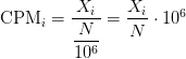
RPKM/FPKM: Controls for sequencing depth and gene length. Good for technical replicates, not good for sample-sample due to compositional bias. Assumes total RNA output is same in all samples. Not for DE.
TPM: Similar to RPKM/FPKM. Corrects for sequencing depth and gene length. Also comparable between samples but no correction for compositional bias.
TMM/RLE/MRN: Improved assumption: The output between samples for a core set only of genes is similar. Corrects for compositional bias. Used for DE. RLE and MRN are very similar and correlates well with sequencing depth. edgeR::calcNormFactors() implements TMM, TMMwzp, RLE & UQ. DESeq2::estimateSizeFactors implements median ratio method (RLE). Does not correct for gene length.
VST/RLOG/VOOM: Variance is stabilised across the range of mean values. For use in exploratory analyses. Not for DE. vst() and rlog() functions from DESeq2. voom() function from Limma converts data to normal distribution.
geTMM: Gene length corrected TMM.
For DEG using DEG R packages (DESeq2, edgeR, Limma etc), use raw counts
For visualisation (PCA, clustering, heatmaps etc), use TPM or TMM
For own analysis with gene length correction, use TPM (maybe geTMM?)
Other solutions: spike-ins/house-keeping genes
Featurecount
featureCounts -p -a <GENOME>.gtf <SAMPLE1>.bam <SAMPLE2>.bam <SAMPLE3>.bam ...... -o counts.txt
micromamba activate RNASEQ_bch709
cd ~/scratch/rnaseq/ATH/bam
featureCounts -o ATH.featureCount.cnt -p --countReadPairs -a ~/scratch/rnaseq/ATH/reference/TAIR10_GFF3_genes.gtf SRR1761506.bamAligned.sortedByCoord.out.bam  SRR1761509.bamAligned.sortedByCoord.out.bam SRR1761507.bamAligned.sortedByCoord.out.bam  SRR1761510.bamAligned.sortedByCoord.out.bam SRR1761508.bamAligned.sortedByCoord.out.bam  SRR1761511.bamAligned.sortedByCoord.out.bam
micromamba activate RNASEQ_bch709
cd ~/scratch/rnaseq/Mmusculus/bam
featureCounts -o Mmusculus.featureCount.cnt -p --countReadPairs -a ~/scratch/rnaseq/Mmusculus/reference/GRCm39_genomic.gtf -g "gene_name"  <YOUR BAM FILES>
FPKM
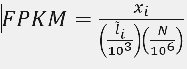
X = mapped reads count N = number of reads L = Length of transcripts
‘length’ is this transcript’s sequence length (poly(A) tail is not counted). ‘effective_length’ counts only the positions that can generate a valid fragment.
FPKM
Fragments per Kilobase of transcript per million mapped reads
X = 3752
Number_Reads_mapped = 559192
Length = 651.04
fpkm= X*(1000/Length)*(1000000/Number_Reads_mapped)
fpkm
ten to the ninth power = 10**9
TPM
Transcripts Per Million
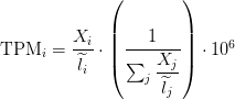
Paper read
FPKM
Fragments per Kilobase of transcript per million mapped reads
awk 'FNR > 2 { sum+=$7 } END {print sum}' ATH.featureCount.cnt
Example AT1G01060.TAIR10
Length = 976
X = 500
Number_Reads_mapped = 5949384
fpkm= X*(1000/Length)*(1000000/Number_Reads_mapped)
fpkm
ten to the ninth power = 10**9
fpkm=X/(Number_Reads_mapped*Length)*10**9
fpkm
TPM
sum_count_per_length
awk 'FNR > 2 { sum+=$7/$6 } END {print sum}' ATH.featureCount.cnt
egrep AT1G01060 ATH.featureCount.cnt
TPM calculation from reads count
sum_count_per_length =  4747.27
X = 500
Length = 976
TPM = (X/Length)*(1/sum_count_per_length )*10**6
TPM
TPM and FPKM calculation
cut -f1,6-  ATH.featureCount.cnt |  egrep -v "#" | sed 's/\Aligned\.sortedByCoord\.out\.bam//g; s/\.bam//g' > ATH.featureCount_count_length.cnt

python /data/gpfs/assoc/bch709-6/Course_material/script/tpm_raw_exp_calculator.py -count ATH.featureCount_count_length.cnt
TPM calculation from FPKM
FPKM = 86.10892858272605
SUM_FPKM = 797942
TPM=(FPKM/SUM_FPKM)*10**6
TPM
Featurecount calculation
Use GTF and BAM file under reference and bam folder, respectively.
Drosophila
Mus musculus
Solanum lycopersicum
Mosquito (Anopheles stephensi)
MultiQC summary
MultiQC walks a directory and stitches every QC artifact (fastp JSON, STAR Log.final.out, featureCounts .summary, FastQC, etc.) into a single HTML report — the one file you open to see whether every sample of the cohort behaved.
Arabidopsis
Save as ~/scratch/rnaseq/ATH/multiqc.sh:
#!/bin/bash
#SBATCH --job-name=multiqc_ATH
#SBATCH --account=cpu-s5-bch709-6
#SBATCH --partition=cpu-core-0
#SBATCH --cpus-per-task=2
#SBATCH --mem=8g
#SBATCH --time=01:00:00
#SBATCH --mail-type=FAIL,END
#SBATCH --mail-user=<YOUR_EMAIL>
#SBATCH -o logs/multiqc_%j.out

set -euo pipefail
cd ~/scratch/rnaseq/ATH

mkdir -p qc

# Pull together everything multiqc can parse under the project dir
multiqc . -o qc/ -n ATH_report --force \
    --module fastp \
    --module star \
    --module featureCounts \
    --exclude rsem \
    --exclude gatk
⚠️ Don’t run bare
multiqc .interactively. Runningmultiqc .from~/scratch/rnaseq/or any parent dir is risky — MultiQC 1.34 has known module-parsing bugs (rsem,gatk) that crash the whole report when stale files from another lesson are picked up. If you must run multiqc interactively, mirror the script’s flag set:# From inside the project dir: cd ~/scratch/rnaseq/ATH multiqc . -o qc/ -n ATH_report --force \ --module fastp --module star --module featureCounts \ --exclude rsem --exclude gatkBetter: just
sbatch multiqc.sh.
What this picks up:
| Module | Source files | What you see |
|---|---|---|
fastp |
trim/*_fastp.json |
Q20/Q30 rates, duplication %, adapter trimming per sample |
star |
bam/*Log.final.out |
Uniquely mapped %, multi-mapped %, splicing rates |
featureCounts |
ATH.featureCount.cnt.summary |
Assigned vs unassigned reads (ambiguity, no-feature, multi-mapping) |
Submit (after align.sh and featureCounts have finished):
MQC_JID=$(sbatch --parsable --dependency=afterany:${FC_JID} multiqc.sh)
echo "MultiQC: ${MQC_JID}"
Once it finishes, copy the report to your laptop and open it in a browser:
scp <netid>@pronghorn.rc.unr.edu:~/scratch/rnaseq/ATH/qc/ATH_report.html ./
open ATH_report.html      # or: double-click in your file browser
Drosophila / Mus musculus / Solanum lycopersicum / Mosquito (Anopheles stephensi)
Same script, only the project path changes — copy multiqc.sh into the species dir and update one line:
cd ~/scratch/rnaseq/Drosophila    # or Mmusculus / Slycopersicum / Astephensi
cp ../ATH/multiqc.sh .
sed -i 's|~/scratch/rnaseq/ATH|~/scratch/rnaseq/Drosophila|g; s|ATH_report|Drosophila_report|g' multiqc.sh
sbatch multiqc.sh
The report will show the same modules as above. If a section is missing, the upstream step’s artifact wasn’t written — check that step’s log before continuing to DE analysis.
DESeq2 vs EdgeR Normalization method
DESeq and EdgeR are very similar and both assume that no genes are differentially expressed. DEseq uses a “geometric” normalisation strategy, whereas EdgeR is a weighted mean of log ratios-based method. Both normalise data initially via the calculation of size / normalisation factors.
Here is further information (important parts in bold):
DESeq
DESeq: This normalization method is included in the DESeq Bioconductor package (version 1.6.0) and is based on the hypothesis that most genes are not DE. A DESeq scaling factor for a given lane is computed as the median of the ratio, for each gene, of its read count over its geometric mean across all lanes. The underlying idea is that non-DE genes should have similar read counts across samples, leading to a ratio of 1. Assuming most genes are not DE, the median of this ratio for the lane provides an estimate of the correction factor that should be applied to all read counts of this lane to fulfill the hypothesis. By calling the estimateSizeFactors() and sizeFactors() functions in the DESeq Bioconductor package, this factor is computed for each lane, and raw read counts are divided by the factor associated with their sequencing lane.
DESeq2
ϕ was assumed to be a function of μ determined by nonparametric regression. The recent version used in this paper follows a more versatile procedure. Firstly, for each transcript, an estimate of the dispersion is made, presumably using maximum likelihood. Secondly, the estimated dispersions for all transcripts are fitted to the functional form:
ϕ=a+bμ(DESeq parametric fit), using a gamma-family generalised linear model (Using regression)
This normalization method is included in the DESeq Bioconductor package and is based on the hypothesis that most genes are not DE. A DESeq scaling factor for a given lane is computed as the median of the ratio, for each gene, of its read count over its geometric mean across all lanes. The underlying idea is that non-DE genes should have similar read counts across samples, leading to a ratio of 1. Assuming most genes are not DE, the median of this ratio for the lane provides an estimate of the correction factor that should be applied to all read counts of this lane to fulfill the hypothesis. By calling the estimateSizeFactors() and sizeFactors() functions in the DESeq Bioconductor package, this factor is computed for each lane, and raw read counts are divided by the factor associated with their sequencing lane.
EdgeR
Trimmed Mean of M-values (TMM): This normalization method is implemented in the edgeR Bioconductor package (version 2.4.0). It is also based on the hypothesis that most genes are not DE. The TMM factor is computed for each lane, with one lane being considered as a reference sample and the others as test samples. For each test sample, TMM is computed as the weighted mean of log ratios between this test and the reference, after exclusion of the most expressed genes and the genes with the largest log ratios. According to the hypothesis of low DE, this TMM should be close to 1. If it is not, its value provides an estimate of the correction factor that must be applied to the library sizes (and not the raw counts) in order to fulfill the hypothesis. The calcNormFactors() function in the edgeR Bioconductor package provides these scaling factors. To obtain normalized read counts, these normalization factors are re-scaled by the mean of the normalized library sizes. Normalized read counts are obtained by dividing raw read counts by these re-scaled normalization factors.
EdgeR
edgeR recommends a “tagwise dispersion” function, which estimates the dispersion on a gene-by-gene basis, and implements an empirical Bayes strategy for squeezing the estimated dispersions towards the common dispersion. Under the default setting, the degree of squeezing is adjusted to suit the number of biological replicates within each condition: more biological replicates will need to borrow less information from the complete set of transcripts and require less squeezing.
Trimmed Mean of M-values (TMM): This normalization method hypothesis that most genes are not DE. The TMM factor is computed for each lane, with one lane being considered as a reference sample and the others as test samples. For each test sample, TMM is computed as the weighted mean of log ratios between this test and the reference, after exclusion of the most expressed genes and the genes with the largest log ratios. According to the hypothesis of low DE, this TMM should be close to 1. If it is not, its value provides an estimate of the correction factor that must be applied to the library sizes (and not the raw counts) in order to fulfill the hypothesis. The calcNormFactors() function in the edgeR Bioconductor package provides these scaling factors. To obtain normalized read counts, these normalization factors are re-scaled by the mean of the normalized library sizes. Normalized read counts are obtained by dividing raw read counts by these re-scaled normalization factors.
DESeq2 vs EdgeR Statistical tests for differential expression
DESeq2
DESeq2 uses raw counts, rather than normalized count data, and models the normalization to fit the counts within a Generalized Linear Model (GLM) of the negative binomial family with a logarithmic link. Statistical tests are then performed to assess differential expression, if any.
EdgeR
Data are normalized to account for sample size differences and variance among samples. The normalized count data are used to estimate per-gene fold changes and to perform statistical tests of whether each gene is likely to be differentially expressed.
EdgeR uses an exact test under a negative binomial distribution (Robinson and Smyth, 2008). The statistical test is related to Fisher’s exact test, though Fisher uses a different distribution.
Major difference
The major differences between the two methods are in some of the defaults. DESeq2 by default does a couple things (which can all optionally be turned off): it finds an optimal value at which to filter low count genes, flags genes with large outlier counts or removes these outlier values when there are sufficient samples per group (n>6), excludes from the estimation of the dispersion prior and dispersion moderation those genes with very high within-group variance, and moderates log fold changes which have small statistical support (e.g. from low count genes). edgeR offers similar functionality, for example, it offers a robust dispersion estimation function, estimateGLMRobustDisp, which reduces the effect of individual outlier counts, and a robust argument to estimateDisp so that hyperparameters are not overly affected by genes with very high within-group variance. And the default steps in the edgeR User Guide for filtering low counts genes both increases power by reducing multiple testing burden and removes genes with uninformative log fold changes.
Fold change
Fold change (FC) is a measure describing the degree of quantity change between control and treatment value. For instance, for a data set with an control of 20 and a treatment of 80, the corresponding fold change is 3, or in common terms, a three-fold increase. Fold change is computed simply as the ratio of the changes between treatment value and the control value over the initial value. Thus, if the control value is X and treatment value is Y, the fold change is (Y - X)/X or equivalently Y/X - 1. As another example, a change from 60 to 30 would be a fold change of -0.5, while a change from 30 to 60 would be a fold change of 1 (a change of 2 times the original).
Likely because of this definition, many researchers use both“fold”and“fold change” to be synonymous with “times,” as in “2-fold larger” = “2 times larger.” Among some experts in this field use persists of fold change as in “40 is 1-fold greater than 20.” Therefore, one could argue that the use of fold change, as in “X is 3-fold greater than 15” should be avoided altogether, since some will interpret this to mean X is 45 whereas others will understand this to mean that A is 60.
In DESeq2 Fold change is typically calculated by simply average of group 2/ average of group 1.
(average in group2)/(average in group1)
The question is why would you want to do this? There are good Bioconductor packages that can do that for you. For example, DESeq2 applies shrinkage methods to the fold-changes. Raw fold-change is not informative in bioinformatic statistical analysis, because it doesn’t address the expression level (and variance) of the gene. Highly and lowly expressed genes can give you the same fold-change, and you don’t want this to happen.
Hypothesis testing using the Wald test
The first step in hypothesis testing is to set up a null hypothesis for each gene. In our case is, the null hypothesis is that there is no differential expression across the two sample groups (LFC == 0). Notice that we can do this without observing any data, because it is based on a thought experiment. Second, we use a statistical test to determine if based on the observed data, the null hypothesis is true. With DESeq2, the Wald test is commonly used for hypothesis testing when comparing two groups. A Wald test statistic is computed along with a probability that a test statistic at least as extreme as the observed value were selected at random. This probability is called the p-value of the test. If the p-value is small we reject the null hypothesis and state that there is evidence against the null (i.e. the gene is differentially expressed).
Multiple test correction
Note that we have pvalues and p-adjusted values in the output. Which should we use to identify significantly differentially expressed genes?
If we used the p-value directly from the Wald test with a significance cut-off of p < 0.05, that means there is a 5% chance it is a false positives. Each p-value is the result of a single test (single gene). The more genes we test, the more we inflate the false positive rate. This is the multiple testing problem. For example, if we test 20,000 genes for differential expression, at p < 0.05 we would expect to find 1,000 genes by chance. If we found 3000 genes to be differentially expressed total, roughly one third of our genes are false positives. We would not want to sift through our “significant” genes to identify which ones are true positives.
DESeq2 helps reduce the number of genes tested by removing those genes unlikely to be significantly DE prior to testing, such as those with low number of counts and outlier samples (gene-level QC). However, we still need to correct for multiple testing to reduce the number of false positives, and there are a few common approaches:
Bonferroni
The adjusted p-value is calculated by: p-value * m (m = total number of tests). This is a very conservative approach with a high probability of false negatives, so is generally not recommended.
FDR/Benjamini-Hochberg
Benjamini and Hochberg (1995) defined the concept of FDR and created an algorithm to control the expected FDR below a specified level given a list of independent p-values. An interpretation of the BH method for controlling the FDR is implemented in DESeq2 in which we rank the genes by p-value, then multiply each ranked p-value by m/rank.
Q-value / Storey method
The minimum FDR that can be attained when calling that feature significant. For example, if gene X has a q-value of 0.013 it means that 1.3% of genes that show p-values at least as small as gene X are false positives
Deafault test
In DESeq2, the p-values attained by the Wald test are corrected for multiple testing using the Benjamini and Hochberg method by default. There are options to use other methods in the results() function. The p-adjusted values should be used to determine significant genes. The significant genes can be output for visualization and/or functional analysis.
So what does FDR < 0.05 mean? By setting the FDR cutoff to < 0.05, we’re saying that the proportion of false positives we expect amongst our differentially expressed genes is 5%. For example, if you call 500 genes as differentially expressed with an FDR cutoff of 0.05, you expect 25 of them to be false positives.
Environment
micromamba create -n DEG_bch709 -c conda-forge -c bioconda -y \
    r-gplots r-fastcluster=1.1.25 \
    bioconductor-ctc bioconductor-deseq2 bioconductor-qvalue \
    bioconductor-limma bioconductor-edger bioconductor-genomeinfodb \
    bioconductor-topgo bioconductor-org.at.tair.db \
    bioconductor-org.mm.eg.db bioconductor-org.hs.eg.db \
    r-rcurl bedtools intervene r-upsetr r-corrplot r-cairo

micromamba activate DEG_bch709
Arabidopsis
| Sample information | Run |
|---|---|
| WT_rep1 | SRR1761506 |
| WT_rep2 | SRR1761507 |
| WT_rep3 | SRR1761508 |
| ABA_rep1 | SRR1761509 |
| ABA_rep2 | SRR1761510 |
| ABA_rep3 | SRR1761511 |
Slycopersium
| Run ID | LibraryName |
|---|---|
| SRR15607542 | Root control Rep1 |
| SRR15607543 | Root control Rep2 |
| SRR15607544 | Root control Rep3 |
| SRR15607552 | Root Salt treatment Rep1 |
| SRR15607553 | Root Salt treatment Rep2 |
| SRR15607554 | Root Salt treatment Rep3 |
Astephensi
| Run ID | LibraryName |
|---|---|
| SRR1851022 | Anopheles stephensi male RNAseq replicate 1 |
| SRR1851024 | Anopheles stephensi male RNAseq replicate 2 |
| SRR1851026 | Anopheles stephensi male RNAseq replicate 3 |
| SRR1851027 | Anopheles stephensi female RNAseq replicate 1 |
| SRR1851028 | Anopheles stephensi female RNAseq replicate 2 |
| SRR1851030 | Anopheles stephensi female RNAseq replicate 3 |
Mmusculus
| Run ID | LibraryName |
|---|---|
| SRR16526489 | Mock 1; Mus musculus; RNA-Seq |
| SRR16526488 | Mock 2; Mus musculus; RNA-Seq |
| SRR16526486 | Mock 3; Mus musculus; RNA-Seq |
| SRR16526483 | Mock 4; Mus musculus; RNA-Seq |
| SRR16526477 | CoV2 3; Mus musculus; RNA-Seq |
| SRR16526479 | CoV2 2; Mus musculus; RNA-Seq |
| SRR16526481 | CoV2 1; Mus musculus; RNA-Seq |
| SRR16526475 | CoV2 4; Mus musculus; RNA-Seq |
Drosophila
| Sample information | Run |
|---|---|
| Control | SRR16287545 |
| Control | SRR16287546 |
| Control | SRR16287547 |
| Ethanol treatment | SRR16287549 |
| Ethanol treatment | SRR16287548 |
| Ethanol treatment | SRR16287550 |
ATH DEG
cd ~/scratch/rnaseq/ATH
mkdir DEG
cd DEG
cp ~/scratch/rnaseq/ATH/bam/ATH.featureCount* .

cut -f1,7- ATH.featureCount.cnt | egrep -v "#" | sed 's/\.bamAligned\.sortedByCoord\.out\.bam//g; s/\.TAIR10//g' > ATH.featureCount_count_only.cnt
Sample file
nano samples.txt
Control<TAB>SRR1761506
Control<TAB>SRR1761507
Control<TAB>SRR1761508
ABA<TAB>SRR1761509
ABA<TAB>SRR1761510
ABA<TAB>SRR1761511
PtR (Quality Check Your Samples and Biological Replicates)
Once you’ve performed transcript quantification for each of your biological replicates, it’s good to examine the data to ensure that your biological replicates are well correlated, and also to investigate relationships among your samples. If there are any obvious discrepancies among your sample and replicate relationships such as due to accidental mis-labeling of sample replicates, or strong outliers or batch effects, you’ll want to identify them before proceeding to subsequent data analyses (such as differential expression).
PtR --matrix ATH.featureCount_count_only.cnt --samples samples.txt --CPM --log2 --min_rowSums 10 --sample_cor_matrix --compare_replicates
Control.rep_compare.pdf
ABA.rep_compare.pdf
DEG calculation
run_DE_analysis.pl --matrix ATH.featureCount_count_only.cnt --method DESeq2 --samples_file samples.txt --output rnaseq
Slycopersium DEG
cd ~/scratch/rnaseq/Slycopersium
mkdir DEG
cd DEG
cp ~/scratch/rnaseq/Slycopersium/bam/Slycopersium.featureCount* .

cut -f1,7- Slycopersium.featureCount.cnt | egrep -v "#" | sed 's/\.bamAligned\.sortedByCoord\.out\.bam//g; s/\.ITAG4\.0//g' > Slycopersium.featureCount_count_only.cnt
Sample file
nano samples.txt
Control SRR15607542
Control SRR15607543
Control SRR15607544
Salt    SRR15607552
Salt    SRR15607553
Salt    SRR15607554
PtR (Quality Check Your Samples and Biological Replicates)
PtR –matrix Slycopersium.featureCount_count_only.cnt –samples samples.txt –CPM –log2 –min_rowSums 10 –sample_cor_matrix –compare_replicates
DEG calculation
run_DE_analysis.pl --matrix Slycopersium.featureCount_count_only.cnt --method DESeq2 --samples_file samples.txt --output rnaseq
Astephensi DEG
cd ~/scratch/rnaseq/Astephensi
mkdir DEG
cd DEG
cp ~/scratch/rnaseq/Astephensi/bam/*.featureCount* .

cut -f1,7- Astephensi.featureCount.cnt | egrep -v "#" | sed 's/\.bamAligned\.sortedByCoord\.out\.bam//g;' > Astephensi.featureCount_count_only.cnt
Sample file
nano samples.txt
Male    SRR1851022
Male    SRR1851024
Male    SRR1851026
Female  SRR1851027
Female  SRR1851028
Female  SRR1851030
PtR (Quality Check Your Samples and Biological Replicates)
PtR –matrix Astephensi.featureCount_count_only.cnt –samples samples.txt –CPM –log2 –min_rowSums 10 –sample_cor_matrix –compare_replicates
DEG calculation
run_DE_analysis.pl --matrix Astephensi.featureCount_count_only.cnt --method DESeq2 --samples_file samples.txt --output rnaseq
Mmusculus DEG
cd ~/scratch/rnaseq/Mmusculus
mkdir DEG
cd DEG
cp ~/scratch/rnaseq/Mmusculus/bam/*.featureCount* .

cut -f1,7- Mmusculus.featureCount.cnt | egrep -v "#" | sed 's/\.bamAligned\.sortedByCoord\.out\.bam//g' > Mmusculus.featureCount_count_only.cnt
Sample file
nano samples.txt
Mock    SRR16526489
Mock    SRR16526488
Mock    SRR16526486
Mock    SRR16526483
CoV SRR16526477
CoV SRR16526479
CoV SRR16526481
CoV SRR16526475
PtR (Quality Check Your Samples and Biological Replicates)
PtR –matrix Mmusculus.featureCount_count_only.cnt –samples samples.txt –CPM –log2 –min_rowSums 10 –sample_cor_matrix –compare_replicates
DEG calculation
run_DE_analysis.pl --matrix Mmusculus.featureCount_count_only.cnt --method DESeq2 --samples_file samples.txt --output rnaseq
Drosophila DEG
cd ~/scratch/rnaseq/Drosophila
mkdir DEG
cd DEG
cp ~/scratch/rnaseq/Drosophila/bam/*.featureCount* .

cut -f1,7- Drosophila.featureCount.cnt | egrep -v "#" | sed 's/\.bamAligned\.sortedByCoord\.out\.bam//g' > Drosophila.featureCount_count_only.cnt
Sample file
nano samples.txt
Control SRR16287545
Control SRR16287546
Control SRR16287547
Ethanol SRR16287550
Ethanol SRR16287548
Ethanol SRR16287549
PtR (Quality Check Your Samples and Biological Replicates)
PtR –matrix Drosophila.featureCount_count_only.cnt –samples samples.txt –CPM –log2 –min_rowSums 10 –sample_cor_matrix –compare_replicates
DEG calculation
run_DE_analysis.pl --matrix Drosophila.featureCount_count_only.cnt --method DESeq2 --samples_file samples.txt --output rnaseq
RNA-Seq subset
DEG subset
cd rnaseq
## 4-fold and p-value 0.01
analyze_diff_expr.pl --samples ~/scratch/rnaseq/ATH/DEG/samples.txt  --matrix ~/scratch/rnaseq/ATH/DEG/ATH.featureCount_count_length.cnt.tpm.tab -P 0.01 -C 2 --output ATH

## 2-fold and p-value 0.01
analyze_diff_expr.pl --samples  ~/scratch/rnaseq/ATH/DEG/samples.txt   --matrix ~/scratch/rnaseq/ATH/DEG/ATH.featureCount_count_length.cnt.tpm.tab -P 0.01 -C 1 --output ATH
DEG output
ATH.matrix.log2.centered.sample_cor_matrix.pdf
ATH.matrix.log2.centered.genes_vs_samples_heatmap.pdf

ATH.featureCount_count_only.cnt.ABA_vs_Control.DESeq2.DE_results.P0.01_C2.ABA-UP.subset
ATH.featureCount_count_only.cnt.ABA_vs_Control.DESeq2.DE_results.P0.01_C2.Control-UP.subset
ATH.featureCount_count_only.cnt.ABA_vs_Control.DESeq2.DE_results.P0.01_C2.DE.subset

ATH.featureCount_count_only.cnt.ABA_vs_Control.DESeq2.DE_results.P0.01_C1.ABA-UP.subset
ATH.featureCount_count_only.cnt.ABA_vs_Control.DESeq2.DE_results.P0.01_C1.Control-UP.subset
ATH.featureCount_count_only.cnt.ABA_vs_Control.DESeq2.DE_results.P0.01_C1.DE.subset
Venn diagram
Intervene installation
mamba install -c bioconda bedtools intervene r-UpSetR=1.4.0 r-corrplot r-Cairo
cd ~/scratch/rnaseq/ATH/DEG/rnaseq
cut -f 1 ATH.featureCount_count_only.cnt.ABA_vs_Control.DESeq2.DE_results.P0.01_C2.ABA-UP.subset |  grep -v sample > DESeq.UP_4fold.subset
cut -f 1 ATH.featureCount_count_only.cnt.ABA_vs_Control.DESeq2.DE_results.P0.01_C2.Control-UP.subset  |  grep -v sample > DESeq.DOWN_4fold.subset

cut -f 1 ATH.featureCount_count_only.cnt.ABA_vs_Control.DESeq2.DE_results.P0.01_C1.ABA-UP.subset |  grep -v sample > DESeq.UP_2fold.subset
cut -f 1 ATH.featureCount_count_only.cnt.ABA_vs_Control.DESeq2.DE_results.P0.01_C1.Control-UP.subset  |  grep -v sample >DESeq.DOWN_2fold.subset
wc -l DESeq*subset
  701 DESeq.DOWN_2fold.subset
  227 DESeq.DOWN_4fold.subset
 1218 DESeq.UP_2fold.subset
  463 DESeq.UP_4fold.subset
 2609 total
intervene venn --type list --save-overlaps -i DESeq.DOWN_2fold.subset DESeq.DOWN_4fold.subset DESeq.UP_2fold.subset DESeq.UP_4fold.subset
intervene upset --type list --save-overlaps -i DESeq.DOWN_2fold.subset DESeq.DOWN_4fold.subset DESeq.UP_2fold.subset DESeq.UP_4fold.subset
Result
cd Intervene_results
ls
Intervene_upset_combinations.txt
Intervene_upset.pdf
Intervene_upset.R
Intervene_venn.pdf
sets
cd sets
0010_DESeq.UP_2fold.txt
0011_DESeq.UP_2fold_DESeq.UP_4fold.txt
1000_DESeq.DOWN_2fold.txt
1100_DESeq.DOWN_2fold_DESeq.DOWN_4fold.txt
Gene Ontology
Gene Ontology project is a major bioinformatics initiative Gene ontology is an annotation system The project provides the controlled and consistent vocabulary of terms and gene product annotations, i.e. terms occur only once, and there is a dictionary of allowed words GO describes how gene products behave in a cellular context A consistent description of gene products attributes in terms of their associated biological processes, cellular components and molecular functions in a species-independent manner Each GO term consists of a unique alphanumerical identifier, a common name, synonyms (if applicable), and a definition Each term is assigned to one of the three ontologies Terms have a textual definition When a term has multiple meanings depending on species, the GO uses a “sensu” tag to differentiate among them (trichome differentiation (sensu Magnoliophyta)
http://geneontology.org/docs/ontology-documentation/
hypergeometric test
The hypergeometric distribution is the lesser-known cousin of the binomial distribution, which describes the probability of k successes in n draws with replacement. The hypergeometric distribution describes probabilities of drawing marbles from the jar without putting them back in the jar after each draw. The hypergeometric probability mass function is given by (using the original variable convention)

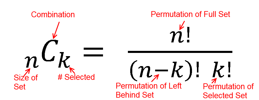
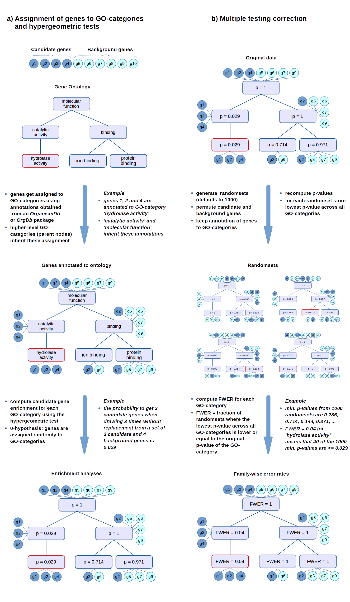
FWER
The FWER for the other tests is computed in the same way: the gene-associated variables (scores or counts) are permuted while the annotations of genes to GO-categories stay fixed. Then the statistical tests are evaluated again for every GO-category.
Hypergeometric Test Example 1
Suppose we randomly select 2 cards without replacement from an ordinary deck of playing cards. What is the probability of getting exactly 2 cards you want (i.e., Ace or 10)?
Solution: This is a hypergeometric experiment in which we know the following:
N = 52; since there are 52 cards in a deck. k = 16; since there are 16 Ace or 10 cards in a deck. n = 2; since we randomly select cards from the deck. x = 2; since 2 of the cards we select are red. We plug these values into the hypergeometric formula as follows:
h(x; N, n, k) = [ kCx ] [ N-kCn-x ] / [ NCn ]
h(2; 52, 2, 16) = [ 16C2 ] [ 48C1 ] / [ 52C2 ]
h(2; 52, 2, 16) = [ 325 ] [ 1 ] / [ 1,326 ]
h(2; 52, 2, 16) = 0.0904977
Thus, the probability of randomly selecting 2 Ace or 10 cards is 9%
| category | probability |
|---|---|
| probability mass f | 0.09049773755656108597285 |
| lower cumulative P | 1 |
| upper cumulative Q | 0.09049773755656108597285 |
| Expectation | 0.6153846153846153846154 |
Hypergeometric Test Example 2
Suppose we have 30 DEGs in human genome (200). What is the probability of getting 10 oncogene?
An oncogene is a gene that has the potential to cause cancer.
Solution: This is a hypergeometric experiment in which we know the following:
N = 200; since there are 200 genes in human genome k = 10; since there are 10 oncogenes in human n = 30; since 30 DEGs x = 5; since 5 of the oncogenes in DEGs.
We plug these values into the hypergeometric formula as follows:
h(x; N, n, k) = [ kCx ] [ N-kCn-x ] / [ NCn ]
h(5; 200, 30, 10) = [ 10C5 ] [ 190C25 ] / [ 200C30 ]
h(5; 200, 30, 10) = [ 252 ] [ 11506192278177947613740456466942 ] / [ 409681705022127773530866523638950880 ]
h(5; 200, 30, 10) = 0.007078
Thus, the probability of oncogene 0.7%.
hypergeometry.png
hypergeometric distribution value
| category | probability |
|---|---|
| probability mass f | 0.0070775932109153651831923063371216961166297 |
| lower cumulative P | 0.99903494867072865323201131115533112651846 |
| upper cumulative Q | 0.0080426445401867119511809951817905695981658 |
| Expectation | 1.5 |
False Discovery Rate (FDR) q-value
The false discovery rate (FDR) is a method of conceptualizing the rate of type I errors in null hypothesis testing when conducting multiple comparisons. FDR-controlling procedures are designed to control the expected proportion of “discoveries” (rejected null hypotheses) that are false (incorrect rejections).
- Benjamini–Yekutieli
- Benjamini–Hochberg
- Bonferroni-Selected–Bonferroni
- Bonferroni and Sidak
Gene ontology
http://geneontology.org/
cleverGO
http://s.tartaglialab.com/page/clever_suite
MetaScape
http://metascape.org/gp/index.html
DAVID
https://david.ncifcrf.gov/
Araport
https://bar.utoronto.ca/thalemine/begin.do
REViGO
http://revigo.irb.hr/
Arabidopsis
cd ~/scratch/rnaseq/ATH/DEG/rnaseq

cat DESeq.DOWN_4fold.subset
cat DESeq.UP_4fold.subset
Mouse
~/scratch/rnaseq/Mmusculus/DEG/rnaseq
 cut -f 1 Mmusculus.featureCount_count_only.cnt.CoV_vs_Mock.DESeq2.DE_results.P0.01_C2.Mock-UP.subset | egrep -v sample
https://reactome.org/PathwayBrowser/#/DTAB=AN&ANALYSIS=MjAyMTExMTcwNjE3MjNfNTU5MTM%253D
Tomato
~/scratch/rnaseq/Slycopersium/DEG/rnaseq
Error, no counts from matrix for Solyc12g017350 at /data/gpfs/home/wyim/scratch/bin/miniconda3/envs/DEG_bch709/bin/analyze_diff_expr.pl line 363, <$fh> line 2.
sed -i 's/\.ITAG4\.0//g' Slycopersium.featureCount_count_length.cnt.tpm.tab

analyze_diff_expr.pl --samples ../samples.txt  --matrix ../Slycopersium.featureCount_count_length.cnt.tpm.tab -P 0.01 -C 2 --output Slycopersium
BLAST
BLAST (Basic Local Alignment Search Tool) is a popular program for searching biosequences against databases. BLAST was developed and is maintained by a group at the National Center for Biotechnology Information (NCBI). Salient characteristics of BLAST are:
Local alignments
BLAST tries to find patches of regional similarity, rather than trying to find the best alignment between your entire query and an entire database sequence.
Ungapped alignments
Alignments generated with BLAST do not contain gaps. BLAST’s speed and statistical model depend on this, but in theory it reduces sensitivity. However, BLAST will report multiple local alignments between your query and a database sequence.
Explicit statistical theory
BLAST is based on an explicit statistical theory developed by Samuel Karlin and Steven Altschul (PNAS 87:2284-2268. 1990) The original theory was later extended to cover multiple weak matches between query and database entry PNAS 90:5873. 1993).
CAUTION: the repetitive nature of many biological sequences (particularly naive translations of DNA/RNA) violates assumptions made in the Karlin & Altschul theory. While the P values provided by BLAST are a good rule-of-thumb for initial identification of promising matches, care should be taken to ensure that matches are not due simply to biased amino acid composition.
CAUTION: The databases are contaminated with numerous artifacts. The intelligent use of filters can reduce problems from these sources. Remember that the statistical theory only covers the likelihood of finding a match by chance under particular assumptions; it does not guarantee biological importance.
Heuristic
BLAST is not guaranteed to find the best alignment between your query and the database; it may miss matches. This is because it uses a strategy which is expected to find most matches, but sacrifices complete sensitivity in order to gain speed. However, in practice few biologically significant matches are missed by BLAST which can be found with other sequence search programs. BLAST searches the database in two phases. First it looks for short subsequences which are likely to produce significant matches, and then it tries to extend these subsequences. A substitution matrix is used during all phases of protein searches (BLASTP, BLASTX, TBLASTN) Both phases of the alignment process (scanning & extension) use a substitution matrix to score matches. This is in contrast to FASTA, which uses a substitution matrix only for the extension phase. Substitution matrices greatly improve sensitivity.
Popular BLAST software
BLASTP
search a Protein Sequence against a Protein Database.
BLASTN
search a Nucleotide Sequence against a Nucleotide Database.
TBLASTN
search a Protein Sequence against a Nucleotide Database, by translating each database Nucleotide sequence in all 6 reading frames.
BLASTX
search a Nucleotide Sequence against a Protein Database, by first translating the query Nucleotide sequence in all 6 reading frames.
BLAST site
https://blast.ncbi.nlm.nih.gov/Blast.cgi https://www.uniprot.org/
Rapidly compare a sequence Q to a database to find all sequences in the database with an score above some cutoff S.
- Which protein is most similar to a newly sequenced one?
- Where does this sequence of DNA originate?
- Speed achieved by using a procedure that typically finds most matches with scores > S.
- Tradeoff between sensitivity and specificity/speed
- Sensitivity – ability to find all related sequences
- Specificity – ability to reject unrelated sequences
Homologous sequence are likely to contain a short high scoring word pair, a seed.
– Unlike Baeza-Yates, BLAST doesn’t make explicit guarantees
BLAST then tries to extend high scoring word pairs to compute maximal high scoring segment pairs (HSPs).
– Heuristic algorithm but evaluates the result statistically.
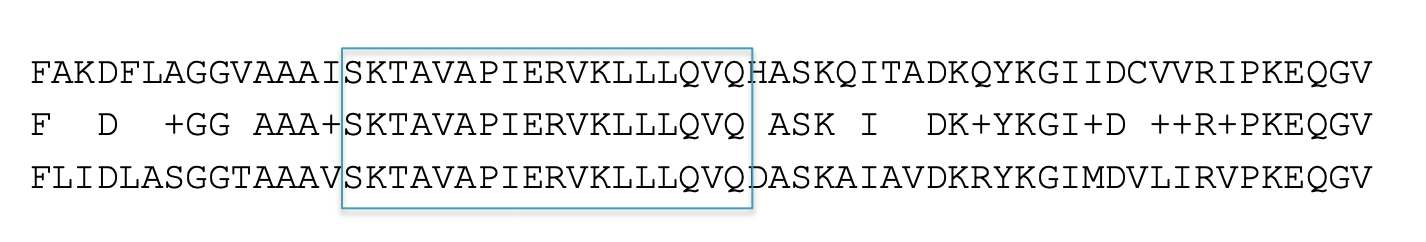
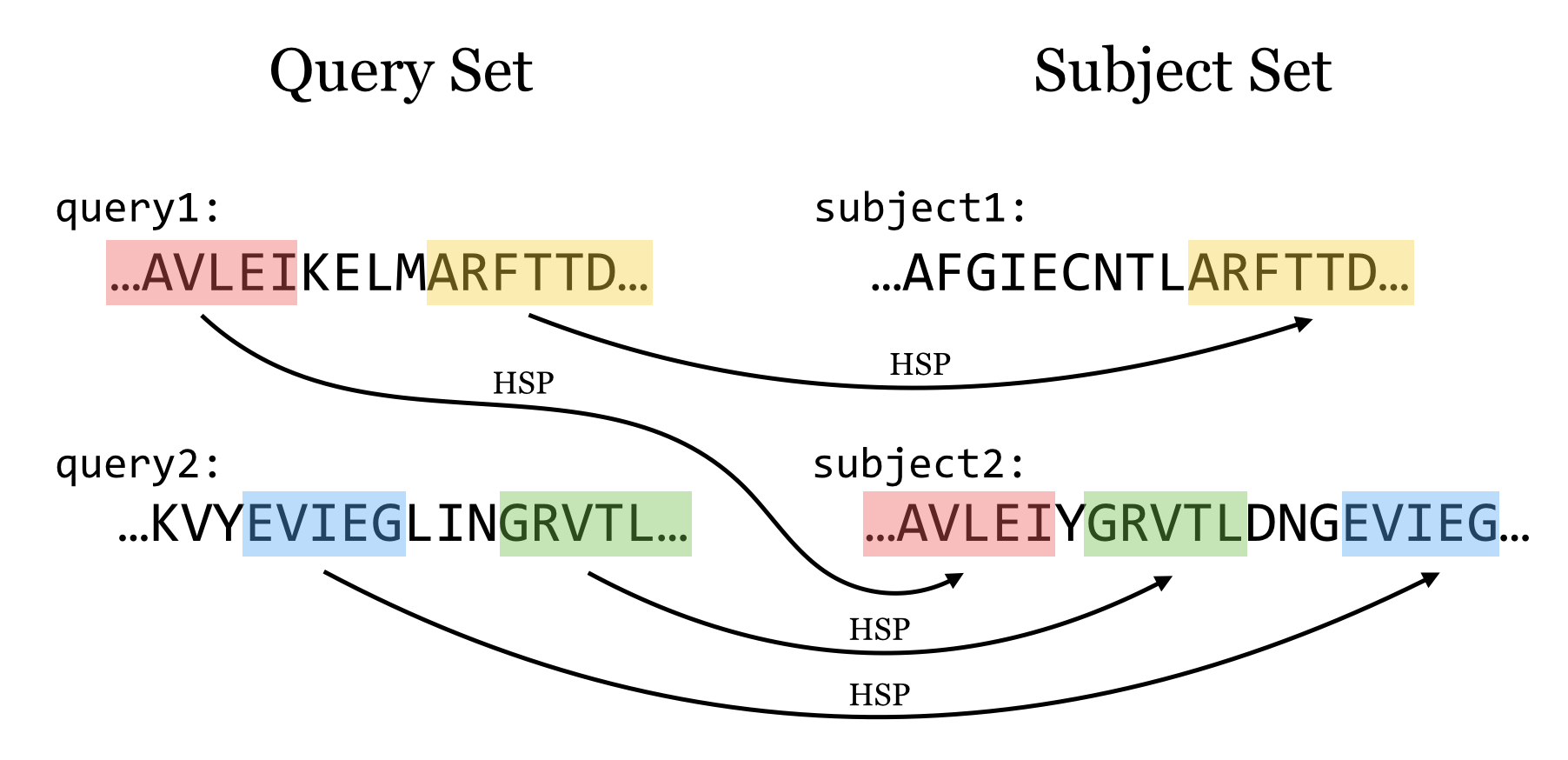
E-value
The Expect value (E) is a parameter that describes the number of hits one can “expect” to see by chance when searching a database of a particular size. It decreases exponentially as the Score (S) of the match increases. Essentially, the E value describes the random background noise.
E-value = the number of HSPs having score S (or higher) expected to occur by chance.
Smaller E-value, more significant in statistics Bigger E-value , by chance
** E[# occurrences of a string of length m in reference of length L] ~ L/4m **
PAM and BLOSUM Matrices
Two different kinds of amino acid scoring matrices, PAM (Percent Accepted Mutation) and BLOSUM (BLOcks SUbstitution Matrix), are in wide use. The PAM matrices were created by Margaret Dayhoff and coworkers and are thus sometimes referred to as the Dayhoff matrices. These scoring matrices have a strong theoretical component and make a few evolutionary assumptions. The BLOSUM matrices, on the other hand, are more empirical and derive from a larger data set. Most researchers today prefer to use BLOSUM matrices because in silico experiments indicate that searches employing BLOSUM matrices have higher sensitivity.
There are several PAM matrices, each one with a numeric suffix. The PAM1 matrix was constructed with a set of proteins that were all 85 percent or more identical to one another. The other matrices in the PAM set were then constructed by multiplying the PAM1 matrix by itself: 100 times for the PAM100; 160 times for the PAM160; and so on, in an attempt to model the course of sequence evolution. Though highly theoretical (and somewhat suspect), it is certainly a reasonable approach. There was little protein sequence data in the 1970s when these matrices were created, so this approach was a good way to extrapolate to larger distances.
Protein databases contained many more sequences by the 1990s so a more empirical approach was possible. The BLOSUM matrices were constructed by extracting ungapped segments, or blocks, from a set of multiply aligned protein families, and then further clustering these blocks on the basis of their percent identity. The blocks used to derive the BLOSUM62 matrix, for example, all have at least 62 percent identity to some other member of the block.
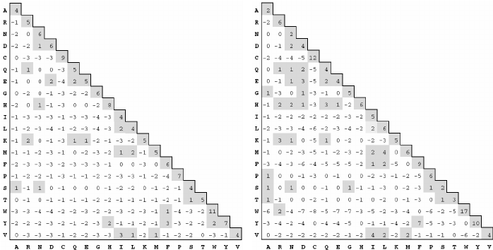
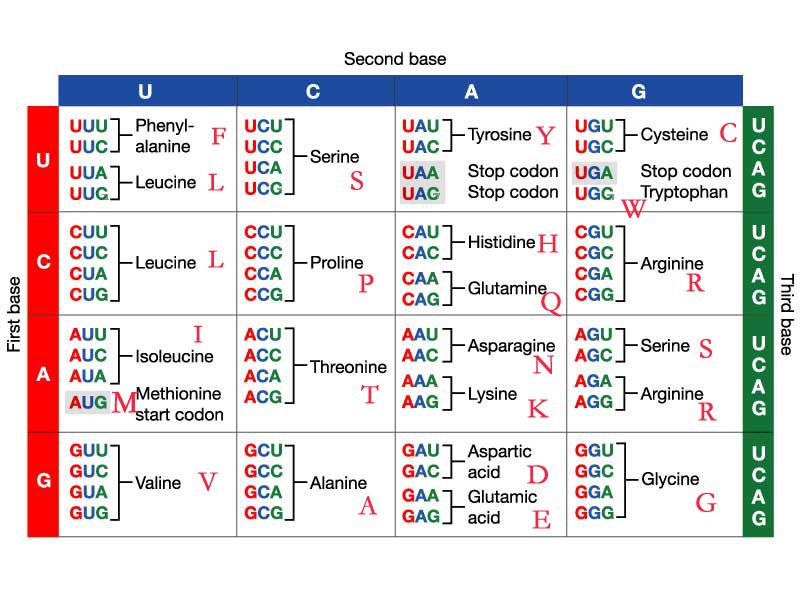
BLAST has a number of possible programs to run depending on whether you have nucleotide or protein sequences:
nucleotide query and nucleotide db - blastn nucleotide query and nucleotide db - tblastx (includes six frame translation of query and db sequences) nucleotide query and protein db - blastx (includes six frame translation of query sequences) protein query and nucleotide db - tblastn (includes six frame translation of db sequences) protein query and protein db - blastp
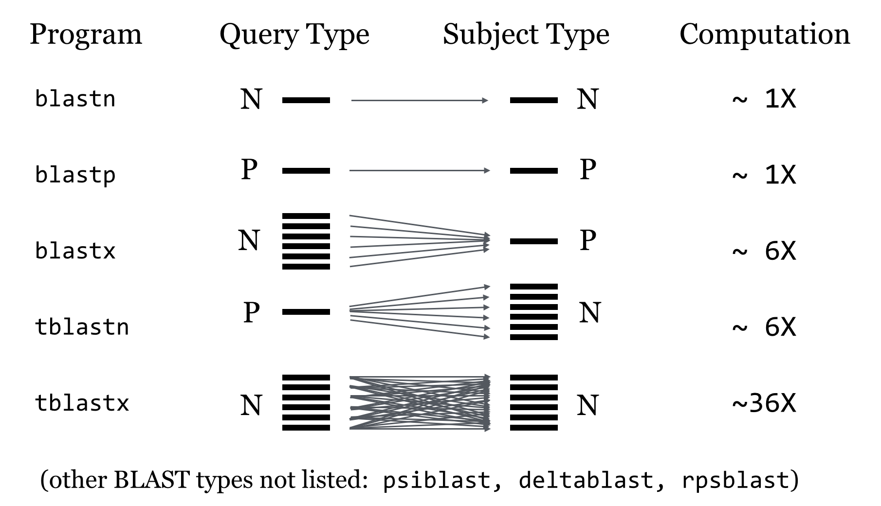
BLAST Process
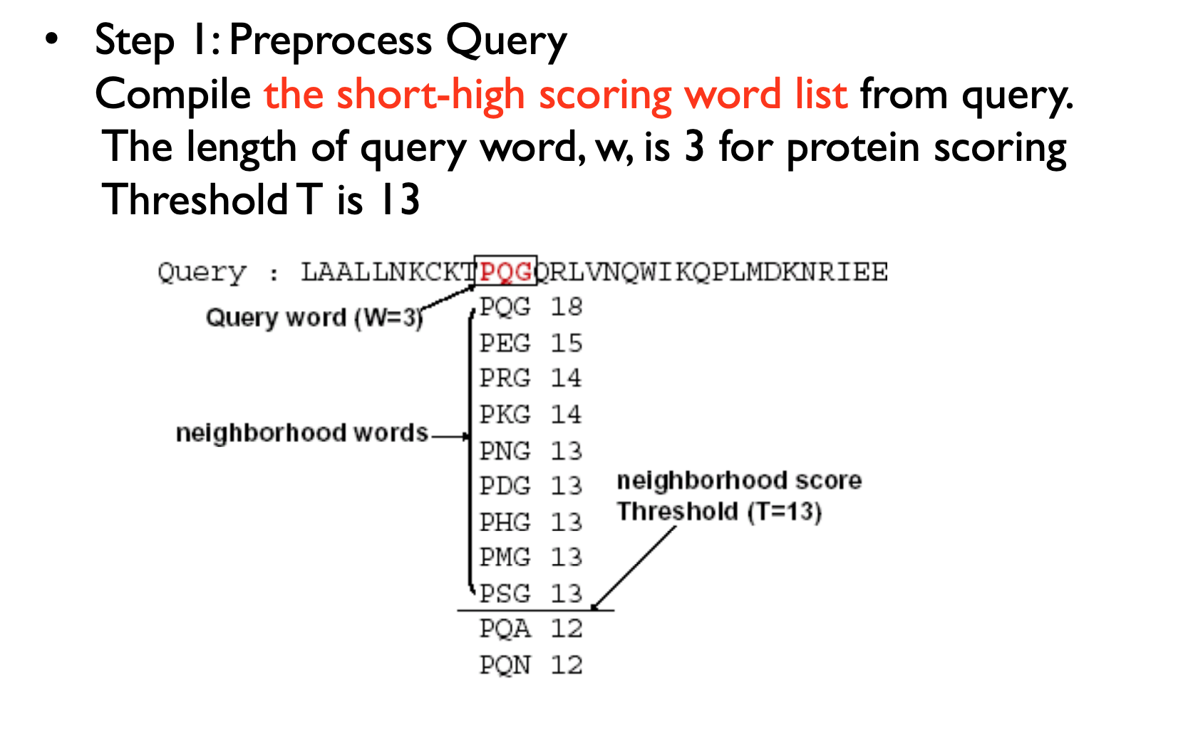
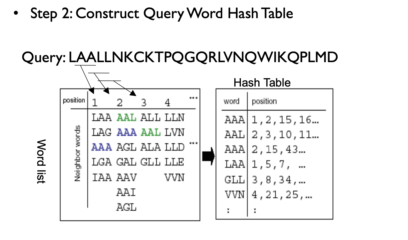
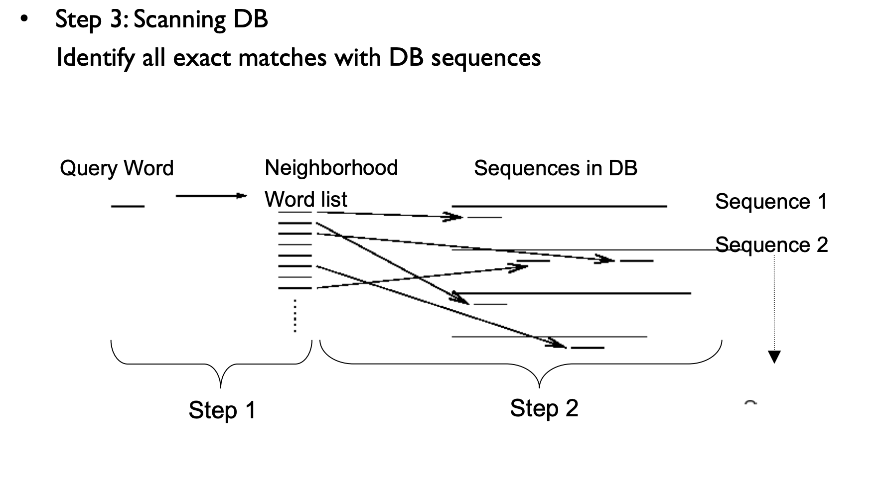
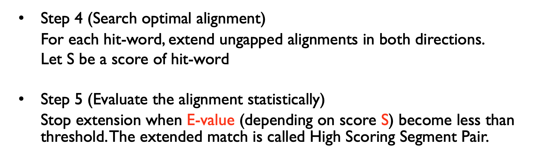
NCBI BLAST
https://blast.ncbi.nlm.nih.gov/Blast.cgi
Uniprot
https://www.uniprot.org/
BLASTN example
Run blastn against the nt database.
ATGAAAGCGAAGGTTAGCCGTGGTGGCGGTTTTCGCGGTGCGCTGAACTA
CGTTTTTGACGTTGGCAAGGAAGCCACGCACACGAAAAACGCGGAGCGAG
TCGGCGGCAACATGGCCGGGAATGACCCCCGCGAACTGTCGCGGGAGTTC
TCAGCCGTGCGCCAGTTGCGCCCGGACATCGGCAAGCCCGTCTGGCATTG
CTCGCTGTCACTGCCTCCCGGCGAGCGCCTGAGCGCCGAGAAGTGGGAAG
CCGTCGCGGCTGACTTCATGCAGCGCATGGGCTTTGACCAGACCAATACG
CCGTGGGTGGCCGTGCGCCACCAGGACACGGACAAGGATCACATCCACAT
CGTGGCCAGCCGGGTAGGGCTGGACGGGAAAGTGTGGCTGGGCCAGTGGG
AAGCCCGCCGCGCCATCGAGGCGACCCAAGAGCTTGAGCATACCCACGGC
CTGACCCTGACGCCGGGGCTGGGCGATGCGCGGGCCGAGCGCCGGAAGCT
GACCGACAAGGAGATCAACATGGCCGTGAGAACGGGCGATGAACCGCCGC
GCCAGCGTCTGCAACGGCTGCTGGATGAGGCGGTGAAGGACAAGCCGACC
GCGCTAGAACTGGCCGAGCGGCTACAGGCCGCAGGCGTAGGCGTCCGGGC
AAACCTCGCCAGCACCGGGCGCATGAACGGCTTTTCCTTCGAGGTGGCCG
GAGTGCCGTTCAAAGGCAGCGACTTGGGCAAGGGCTACACATGGGCGGGG
CTACAGAAAGCAGGGGTGACTTATGACGAAGCTAGAGACCGTGCGGGCCT
TGAACGATTCAGGCCCACAGTTGCAGATCGTGGAGAGCGTCAGGACGTTG
CAGCAGTCCGTGAGCCTGATGCACGAGGACTTGAAGCGCCTACCGGGCGC
AGTCTCGACCGAGACGGCGCAGACCTTGGAACCGCTGGCCCGACTCCGGC
AGGACGTGACGCAGGTTCTGGAAGCCTACGACAAGGTGACGGCCATTCAG
CGCAAGACGCTGGACGAGCTGACGCAGCAGATGAGCGCGAGCGCGGCGCA
GGCCTTCGAGCAGAAGGCCGGGAAGCTGGACGCGACCATCTCCGACCTGT
CGCGCAGCCTGTCAGGGCTGAAAACGAGCCTCAGCAGCATGGAGCAGACC
GCGCAGCAGGTGGCGACCTTGCCGGGCAAGCTGGCGAGCGCACAGCAGGG
CATGACGAAAGCCGCCGACCAACTGACCGAGGCAGCGAACGAGACGCGCC
CGCGCCTTTGGCGGCAGGCGCTGGGGCTGATTCTGGCCGGGGCCGTGGGC
GCGATGCTGGTAGCGACTGGGCAAGTCGCTTTAAACAGGCTAGTGCCGCC
AAGCGACGTGCAGCAGACGGCAGACTGGGCCAACGCGATTTGGAACAAGG
CCACGCCCACGGAGCGCGAGTTGCTGAAACAGATCGCCAATCGGCCCGCG
AACTAGACCCGACCGCCTACCTTGAGGCCAGCGGCTACACCGTGAAGCGA
GAAGGGCGGCACCTGTCCGTCAGGGCGGGCGGTGATGAGGCGTACCGCGT
GACCCGGCAGCAGGACGGGCGCTGGCTCTGGTGCGACCGCTACGGCAACG
ACGGCGGGGACAATATCGACCTGGTGCGCGAGATCGAACCCGGCACCGGC
TACGCCGAGGCCGTCTATCGGCTTTCAGGTGCGCCGACAGTCCGGCAGCA
ACCGCGCCCGAGCGAGCCGAAGCGCCAACCGCCGCAGCTACCGGCGCAAG
GGCTGGCAGCCCGCGAGCATGGCCGCGACTACCTCAAGGGCCGGGGCATC
AGCCAGGACACCATCGAGCACGCCGAGAAGGCGGGCATGGTGCGCTATGC
AGACGGTGGAGTGCTGTTCGTCGGCTACGACCGTGCAGGCACCGCGCAGA
ACGCCACACGCCGCGCCATTGCCCCCGCTGACCCGGTGCAGAAGCGCGAC
CTACGCGGCAGCGACAAGAGCTATCCGCCGATCCTGCCGGGCGACCCGGC
AAAGGTCTGGATCGTGGAAGGTGGCCCGGATGCGCTGGCCCTGCACGACA
TCGCCAAGCGCAGCGGCCAGCAGCCGCCCACCGTCATCGTGTCAGGCGGG
GCGAACGTGCGCAGCTTCTTGGAGCGGGCCGACGTGCAAGCGATCCTGAA
GCGGGCCGAGCGCGTCACCGTGGCCGGGGAAAACGAGAAGAACCCCGAGG
CGCAGGCAAAGGCCGACGCCGGGCACCAGAAGCAGGCGCAGCGGGTGGCC
AAAATCACCGGGCGCGAGGTGCGCCAATGGACGCCGAAGCCCGAGCACGG
CAAGGACTTGGCCGACATGAACGCCCGGCAGGTGGCAGAGATCGAGCGCA
AGCGACAGGCCGAGATCGAGGCCGAAAGAGCACGAAACCGCGAGCTTTCA
CGCAAGAGCCGGAGGTATGATGGCCCCAGCTTCGGCAGATAA
BLASTP Query
Do a BLASTP on NCBI website with the following protein against nr, but limit the organism to cetartiodactyla using default parameters:
MASGPGGWLGPAFALRLLLAAVLQPVSAFRAEFSSESCRELGFSSNLLCSSCDLLGQFSL
LQLDPDCRGCCQEEAQFETKKYVRGSDPVLKLLDDNGNIAEELSILKWNTDSVEEFLSEK
LERI
Have a look at the multiple sequence alignment, can you explain the results?
Do a similar blastp vs UniProtKB (UniProt) without post filtering.
Running a standalone BLAST program
location
mkdir -p ~/scratch/rnaseq/BLAST
cd ~/scratch/rnaseq/BLAST
ENV
micromamba create -n blast -c conda-forge -c bioconda \
    perl-path-tiny blast perl-data-dumper perl-config-tiny seqkit -y
micromamba activate blast
Running a standalone BLAST program
Create the index for the target database using makeblastdb; Choose the task program: blastn, blastp, blastx, tblastx, psiblast or deltablast; Set the configuration for match, mismatch, gap-open penalty, gap-extension penalty or scoring matrix; Set the word size; Set the E-value threshold; Set the output format and the number of output results
Standalone BLAST
In addition to providing BLAST sequence alignment services on the web, NCBI also makes these sequence alignment utilities available for download through FTP. This allows BLAST searches to be performed on local platforms against databases downloaded from NCBI or created locally. These utilities run through DOS-like command windows and accept input through text-based command line switches. There is no graphic user interface
https://www.ncbi.nlm.nih.gov/books/NBK52640/
ftp://ftp.ncbi.nlm.nih.gov/blast/db/
NR vs NT
At NCBI they are two different things as well. ‘nr’ is a database of protein sequences and ‘nt’ is nucleotide. At one time ‘nr’ meant non-redundant but it stopped being non-redundant a while ago. nt is a nucleotide database, while nr is a protein database (in amino acids)
Standalone BLAST
- Download the database.
- Use makeblastdb to build the index.
- Change the scoring matrix, record the changes in the alignment results and interpret the results.
How many sequences in plant.1.protein.faa.gz
Subsampling by SeqKit
FASTA and FASTQ are basic and ubiquitous formats for storing nucleotide and protein sequences. Common manipulations of FASTA/Q file include converting, searching, filtering, deduplication, splitting, shuffling, and sampling. Existing tools only implement some of these manipulations, and not particularly efficiently, and some are only available for certain operating systems. Furthermore, the complicated installation process of required packages and running environments can render these programs less user friendly.
This project describes a cross-platform ultrafast comprehensive toolkit for FASTA/Q processing. SeqKit provides executable binary files for all major operating systems, including Windows, Linux, and Mac OS X, and can be directly used without any dependencies or pre-configurations. SeqKit demonstrates competitive performance in execution time and memory usage compared to similar tools. The efficiency and usability of SeqKit enable researchers to rapidly accomplish common FASTA/Q file manipulations.
https://bioinf.shenwei.me/seqkit/
https://bioinf.shenwei.me/seqkit/tutorial/
Download Database
mkdir -p ~/scratch/rnaseq/BLAST
cd ~/scratch/rnaseq/BLAST
# --retry-all-errors + -C -: harden against SSL eof drops on large
# transfers; resume partials. See HPC_RNA_SEQ.md fastq-dump (#64).
curl -fsSL --retry 5 --retry-all-errors --max-time 600 -C - -O https://ftp.ncbi.nlm.nih.gov/refseq/release/plant/plant.1.protein.faa.gz
Run BLASTX
cd ~/scratch/rnaseq/BLAST
gunzip plant.1.protein.faa.gz
makeblastdb -in plant.1.protein.faa -dbtype prot
seqkit sample -n 100 /data/gpfs/assoc/bch709-6/Course_material/test_mrna.fna > test_mrna.fasta
seqkit sample -n 100 plant.1.protein.faa > test_protein.fasta
blastx -query test_mrna.fasta  -db plant.1.protein.faa
blastx -query test_mrna.fasta  -db plant.1.protein.faa -outfmt 7
Run BLASTP
blastp -query test_protein.fasta -db plant.1.protein.faa -outfmt 7
Run BLASTN
makeblastdb -in test_mrna.fasta -dbtype nucl
blastn -query test_mrna.fasta  -db test_mrna.fasta -outfmt 7 -out blastn.output
Tab output
qseqid      Query sequence ID
sseqid      Subject (ie DB) sequence ID
pident      Percent Identity across the alignment
length      Alignment length
mismatch    # of mismatches
gapopen     Number of gap openings
qstart      Start of alignment in query
qend        End of alignment in query
sstart      Start of alignment in subject
send        End of alignment in subject
evalue      E-value
bitscore    Bit score
DCBLAST
The Basic Local Alignment Search Tool (BLAST) is by far best the most widely used tool in for sequence analysis for rapid sequence similarity searching among nucleic acid or amino acid sequences. Recently, cluster, HPC, grid, and cloud environmentshave been are increasing more widely used and more accessible as high-performance computing systems. Divide and Conquer BLAST (DCBLAST) has been designed to perform run on grid system with query splicing which can run National Center for Biotechnology Information (NCBI) BLASTBLAST search comparisons over withinthe cluster, grid, and cloud computing grid environment by using a query sequence distribution approach NCBI BLAST. This is a promising tool to accelerate BLAST job dramatically accelerates the execution of BLAST query searches using a simple, accessible, robust, and practical approach.
- DCBLAST can run BLAST job across HPC.
- DCBLAST suppport all NCBI-BLAST+ suite.
- DCBLAST generate exact same NCBI-BLAST+ result.
- DCBLAST can use all options in NCBI-BLAST+ suite.
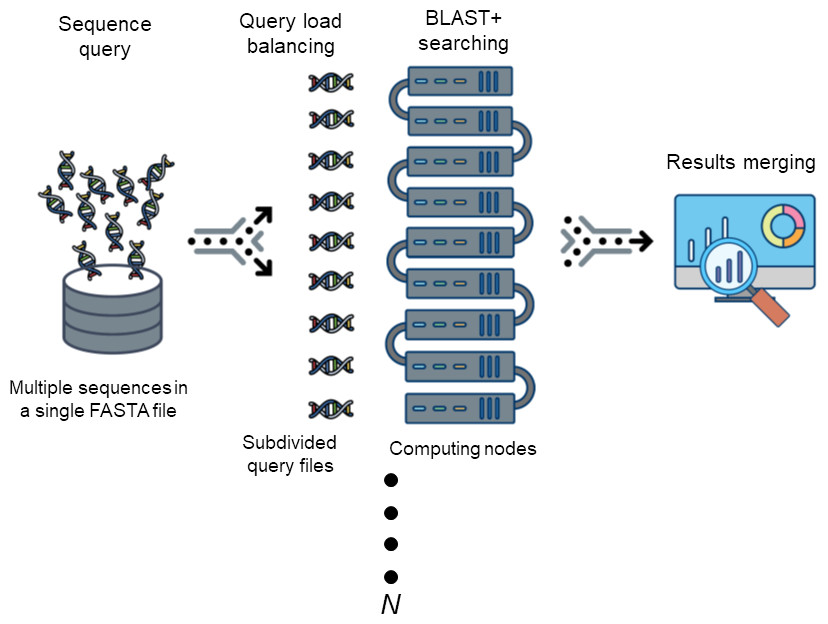
Citation
Won C. Yim and John C. Cushman (2017) Divide and Conquer BLAST: using grid engines to accelerate BLAST and other sequence analysis tools. PeerJ 10.7717/peerj.3486 https://peerj.com/articles/3486/
Ortholog
Example 1
Example 2
Synteny
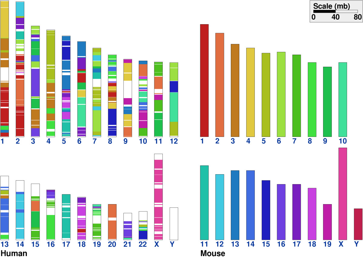
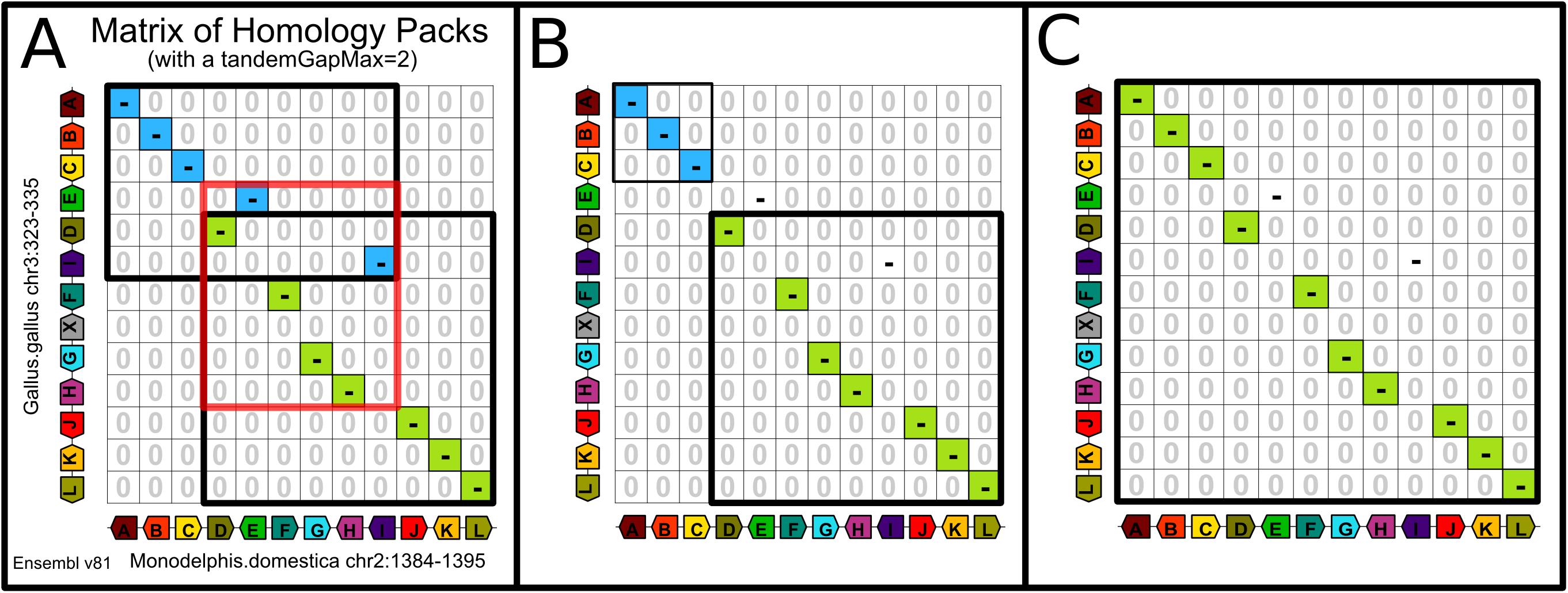
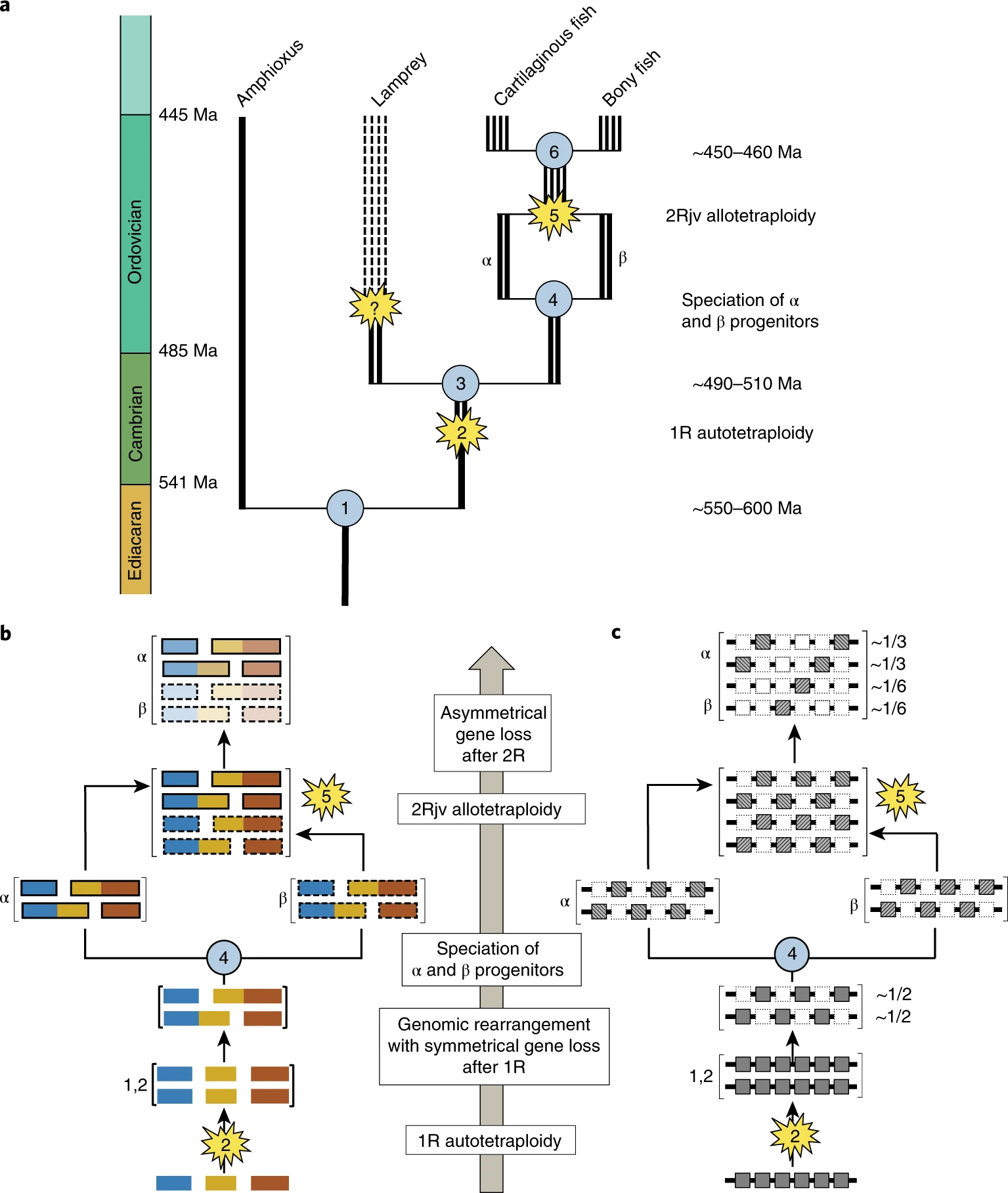
Genome Evolution
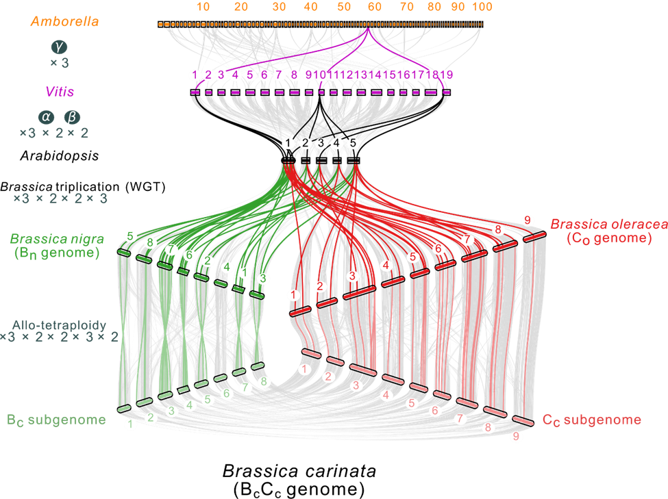
Chromosomal Evolution
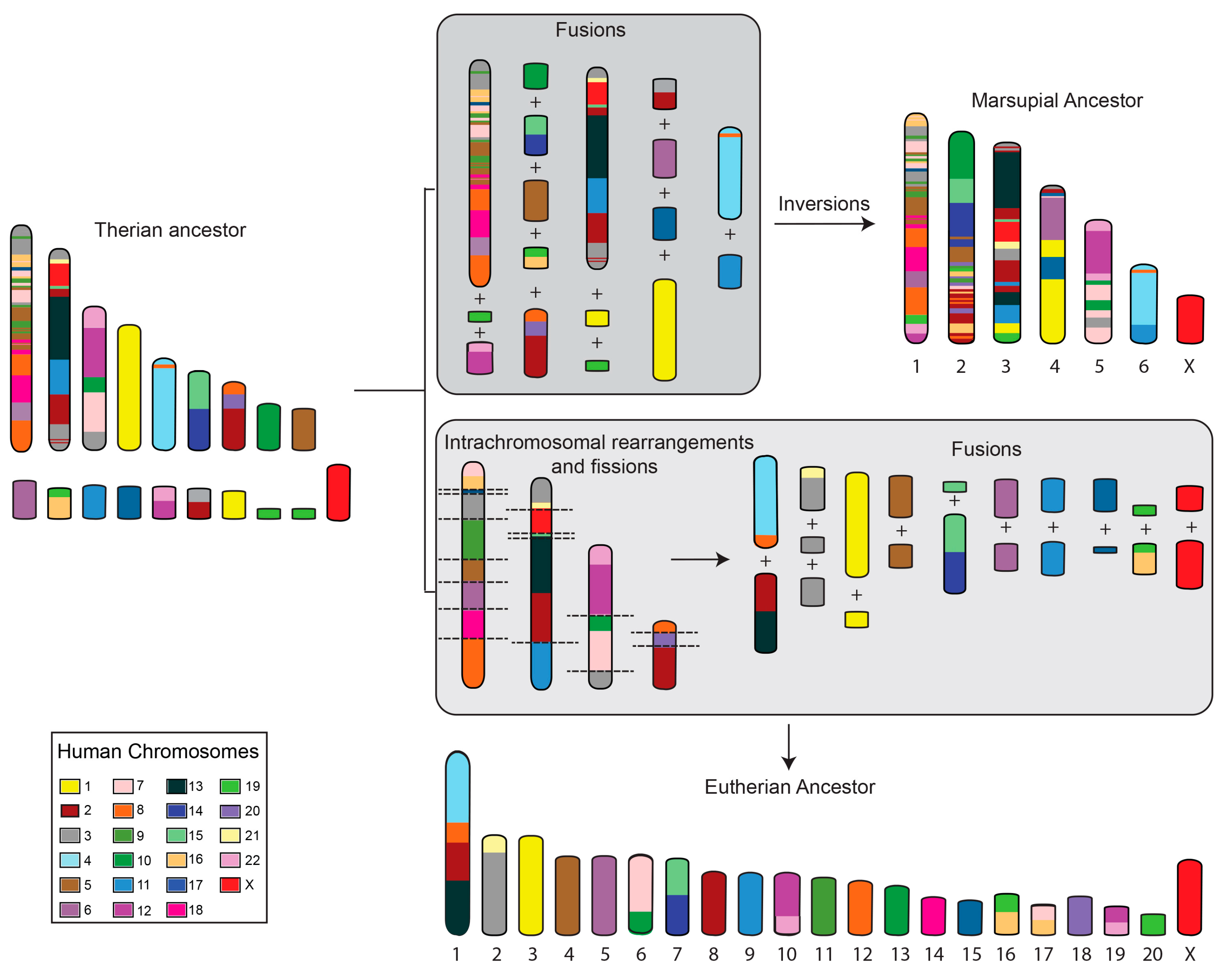
GO Enrichment with topGO (on Pronghorn)
After you have the up/down gene lists from DESeq2, run GO enrichment directly on Pronghorn. topGO is already available in the DEG_bch709 environment used earlier in this lesson.
Prepare the gene lists
# Working directory: your DEG output folder
cd ~/scratch/rnaseq/ATH/DEG/rnaseq/venn

# Universe = every gene tested (from the TPM matrix)
cut -f 1 ../ATH.featureCount_count_length.cnt.tpm.tab | grep -v sample > universe.txt

# Interesting gene set (change file as needed)
cp DESeq.UP_4fold.subset interesting_genes.txt

wc -l universe.txt interesting_genes.txt
Run topGO
Create go_enrichment.R:
# go_enrichment.R
library(topGO)
library(org.At.tair.db)   # change to org.Hs.eg.db / org.Mm.eg.db for human / mouse

args <- commandArgs(trailingOnly = TRUE)
universe_file     <- args[1]   # all genes tested
interesting_file  <- args[2]   # DEGs
out_prefix        <- args[3]   # output prefix

universe    <- readLines(universe_file)
interesting <- readLines(interesting_file)

gene_list <- factor(as.integer(universe %in% interesting))
names(gene_list) <- universe

run_ontology <- function(ont) {
    godata <- new("topGOdata",
                   ontology = ont,
                   allGenes = gene_list,
                   annot = annFUN.org,
                   mapping = "org.At.tair.db",
                   ID = "tair")
    result <- runTest(godata, algorithm = "classic", statistic = "fisher")
    table  <- GenTable(godata,
                       classicFisher = result,
                       topNodes = 30,
                       orderBy = "classicFisher")
    write.table(table,
                file = paste0(out_prefix, "_", ont, ".tsv"),
                sep = "\t", quote = FALSE, row.names = FALSE)
    cat("Wrote", paste0(out_prefix, "_", ont, ".tsv"), "\n")
}

for (ont in c("BP", "MF", "CC")) run_ontology(ont)
Submit as a Slurm job
go_enrichment.sh:
#!/bin/bash
#SBATCH --job-name=go_enrich
#SBATCH --account=cpu-s5-bch709-6
#SBATCH --partition=cpu-core-0
#SBATCH --cpus-per-task=2
#SBATCH --mem=8g
#SBATCH --time=01:00:00
#SBATCH --mail-type=FAIL,END
#SBATCH --mail-user=<YOUR_EMAIL>
#SBATCH -o go_enrich_%j.out

# Activate `DEG_bch709` in your login shell BEFORE running `sbatch go_enrichment.sh`
cd ~/scratch/rnaseq/ATH/DEG/rnaseq/venn

Rscript go_enrichment.R universe.txt interesting_genes.txt ATH_UP4fold
Submit:
sbatch go_enrichment.sh
The output is three tab-separated files per input list — <prefix>_BP.tsv, _MF.tsv, _CC.tsv — with the top 30 GO terms, Fisher p-values, and counts. Copy them to your laptop with rsync and open in Excel or a spreadsheet.
Visualize DEGs — Heatmap and Volcano Plot
Heatmap of top 50 DEGs
heatmap.R:
library(pheatmap)

counts  <- read.table("ATH.featureCount_count_length.cnt.tpm.tab",
                      header = TRUE, row.names = 1, sep = "\t")
deg_ids <- read.table("DEG_ids.txt", header = FALSE)[,1]

mat <- log2(as.matrix(counts[deg_ids, ]) + 1)
mat <- mat[order(-rowMeans(mat)), ][1:min(50, nrow(mat)), ]

pdf("heatmap_top50.pdf", height = 10, width = 7)
pheatmap(mat, scale = "row", show_rownames = TRUE,
         main = "Top 50 DEGs (log2 TPM, row-scaled)")
dev.off()
Volcano plot
volcano.R:
library(ggplot2)

d <- read.table("ATH.featureCount_count_only.cnt.ABA_vs_WT.DESeq2.DE_results",
                 header = TRUE, sep = "\t")
d$sig <- with(d, ifelse(padj < 0.01 & abs(log2FoldChange) >= 2,
                         ifelse(log2FoldChange > 0, "UP", "DOWN"), "NS"))

ggplot(d, aes(log2FoldChange, -log10(pvalue), color = sig)) +
    geom_point(alpha = 0.6, size = 1) +
    scale_color_manual(values = c(UP = "firebrick", DOWN = "steelblue", NS = "grey70")) +
    geom_vline(xintercept = c(-2, 2), linetype = "dashed") +
    geom_hline(yintercept = -log10(0.01), linetype = "dashed") +
    theme_classic() +
    labs(x = "log2 FC (ABA vs WT)", y = "-log10 p-value")

ggsave("volcano.pdf", width = 6, height = 5)
Run either script interactively on Pronghorn:
micromamba activate DEG_bch709
Rscript heatmap.R
Rscript volcano.R
Then copy the PDFs back to your laptop with rsync.
Full RNA-Seq Workflow Summary
| Step | Tool | Script / Section | Output |
|---|---|---|---|
| Download FASTQ | curl from ENA |
fastq-dump.sh | *.fastq.gz |
| QC | FastQC + MultiQC | built-in | HTML report |
| Trim | fastp | trim.sh | Trimmed FASTQ |
| Index | STAR | index.sh | STAR index dir |
| Align | STAR | align.sh | Aligned BAM |
| Count | featureCounts | built-in (align.sh) | *.cnt matrix |
| Normalize | perl (TPM/FPKM) | built-in | TPM/FPKM table |
| DEG | DESeq2 / edgeR (Trinity wrappers) | DEG calculation | *.DE_results |
| Subset DEGs | analyze_diff_expr.pl |
built-in | .subset files |
| Venn overlap | intervene | Draw Venn Diagram | Intervene_* |
| GO enrichment | topGO | go_enrichment.R (above) | *_BP/MF/CC.tsv |
| Visualization | pheatmap / ggplot2 | heatmap.R / volcano.R | .pdf |
Cleanup
# Inside ~/scratch/rnaseq you can remove:
#   - Raw FASTQ (once alignment + trim QC are reviewed)
#   - STAR alignment intermediates (_STARtmp, Log.out, ReadsPerGene.out.tab)
# Keep:
#   - Final BAMs, count matrices, DESeq2/edgeR results, DEG subsets, GO tables, plots

# Example: drop raw FASTQ and STAR tmp (limit scope to ~/scratch/rnaseq)
find ~/scratch/rnaseq -name "*_STARtmp" -type d -exec rm -rf {} +
find ~/scratch/rnaseq -name "*.fastq.gz" -path "*/raw_data/*" -delete
Leaving the Pronghorn session:
micromamba deactivate
exit
Next Steps
- Pathway analysis: feed the DEG list into KEGG or Reactome via their web portals, or use
clusterProfilerin R. - Functional summary: run REViGO on the topGO output to collapse redundant GO terms into a treemap.
- Synteny / ortholog mapping: use the BLAST results from this lesson together with MCScanX for genome-scale comparisons.
- Cross-condition comparison: the intervene UpSet plot shows overlap across 2-fold vs 4-fold cuts in one condition. For two conditions, simply add more
*.subsetfiles beforeintervene venn.