Course Evaluation
Students will have access to course evaluation You can log in with your NetID to http://www.unr.edu/evaluate and check live updating response rates for your course evaluations. Our institutional goal is to achieve an 85% response rate for all evaluations, and to help us achieve that, we rely on you as well as the students.
If we can achieve 100% response rate for evaluation, I will give you additional points for all of you.
Discussion is open
https://unr.canvaslms.com/courses/56453/discussion_topics/514795
The due date for the question is November 23rd 11:59pm The due date for discussion is December 4th 11:59pm
-
Define the biological hypotheses or bottleneck you wish to address which is related to your research, state the approach of your experiment, also state your system, study organism, or study site, and provide justification for what is the goal of your biological hypotheses. Please provide enough background information that the other students can understand your biological hypotheses or bottleneck. If your experiments are complicated, consider briefly explaining the experimental design with reason. If you get more like will get points. (30 Points)
-
Please provide the bioinformatics suggestion that you want to suggest for other people’s research hypotheses or bottleneck. It should be scientifically valid methods even if it does not exist. Provide enough information to create an experiment and if you want to create software, please provide reasons and explain what kind of software we need, which part of the hypotheses or bottleneck can be solved. If the software doesn’t exist, please provide the design or roadmap of your software. Citation is optional but recommended. Please provide an obstacle to other people’s suggestions. In addition, insights and addition will also get points. If you get more like will get points. (10 points per valid answer with reference or concept or hypothesis, a total of 70 Points, seven replies are needed )
3. The suggestion needs to reply as threaded format.
Examples are below
Example
Tef (or Teff) is a warm season, C4-photosynthesis grass that is gaining popularity in the U.S. as a high-quality summer forage, fodder, and gluten-free grain. However, Tef has relatively tiny seeds compare to other C4 grass. Currently, the primary goal of my research is to determine the loci of seed color and size. We are trying to use Genome-wide Association Study (GWAS) https://en.wikipedia.org/wiki/Genome-wide_association_study) (Links to an external site.) to identify the locus of seed color and size. In our lab, we have 386 teff accession and all of them have different seed colors. We extracted all of 386 teff accession DNA and sequencing was done. But I don’t know how to check the size and colors. The phenotyping is the most important but the main bottleneck of our experiment. How can we facilitate this task?
Student A (This example answer will get 3 points) I cannot find any solution but you can use a similar approach such as colony counting. The accurate counting of plates with high numbers of CFUs is error-prone since it requires a high level of attention by the counter. In the microbiome and general biology field use colony count software to analyze whole plate count. The examples are below.
https://www.nature.com/articles/s41598-018-24916-9 (Links to an external site.)
http://opencfu.sourceforge.net/ (Links to an external site.)
Student B (This example answer will get 5 points) I found one software, especially for seed size and color. GrainScan software was designed for seed size and color estimation. GrainScan uses a grayscale image is derived from the scanned color image by converting Red and Green color channel averaging. Based on the grayscaled image, the dimension measurements will be provided which include area, perimeter, and surrogates for length and width the major and minor axes of the best fit ellipse. Another great point of this software will provide color measurements for each seed in CIELAB values based on user provide color calibration options.
https://plantmethods.biomedcentral.com/articles/10.1186/1746-4811-10-23 (Links to an external site.)
Student C (This example answer will get 5 points) I don’t know how to code python, but there are several image analysis packages such as scikit-image (Links to an external site.)
Base on scikit software, you can calculate circularity with “4 * pi * props.area / props.perimeter ** 2”
The props area can be calculated with number of pixels from the centroid approach. The axis location and length can be converted by using orientation value from props and axis value can be estimated cos(orientation) * length/ 2 and sin (orientation) * length/ 2.
Assignment
Please upload three dot plot from assembly comparison.
-
Download below file. https://www.dropbox.com/s/xpnhj6j99dr1kum/Athaliana_subset_bch709-1.fa
-
Align three fasta files (spades_illumina.fasta, spades_pacbio_illumina.fasta, canu.contigs.fasta) to downloaded Athaliana_subset_bch709-1.fa by nucmer independently.
-
Generate coords and coords.idx file using DotPrep.py.
-
Draw dot plot by DOT website.
-
Upload three dotplot to Webcanvas.
wget https://www.dropbox.com/s/xpnhj6j99dr1kum/Athaliana_subset_bch709-1.fa
Install Global Alignmnet Software
cd /data/gpfs/assoc/bch709-1/<YOURID>/Genome_assembly/
mkdir genomeassembly_alignment/
cd genomeassembly_alignment
conda activate genomeassembly
conda install  -c conda-forge -c anaconda -c bioconda mummer -y
Open source MUMmer 3.0 is described in “Versatile and open software for comparing large genomes.” S. Kurtz, A. Phillippy, A.L. Delcher, M. Smoot, M. Shumway, C. Antonescu, and S.L. Salzberg, Genome Biology (2004), 5:R12.
MUMmer 2.1, NUCmer, and PROmer are described in “Fast Algorithms for Large-scale Genome Alignment and Comparision.” A.L. Delcher, A. Phillippy, J. Carlton, and S.L. Salzberg, Nucleic Acids Research (2002), Vol. 30, No. 11 2478-2483.
MUMmer 1.0 is described in “Alignment of Whole Genomes.” A.L. Delcher, S. Kasif, R.D. Fleischmann, J. Peterson, O. White, and S.L. Salzberg, Nucleic Acids Research, 27:11 (1999), 2369-2376.
Space efficent suffix trees are described in “Reducing the Space Requirement of Suffix Trees.” S. Kurtz, Software-Practice and Experience, 29(13): 1149-1171, 1999.
Run Genome Wide Global Alignmnet Software
#!/bin/bash
#SBATCH --job-name=nucmer
#SBATCH --cpus-per-task=2
#SBATCH --time=15:00
#SBATCH --mem=10g
#SBATCH --mail-type=all
#SBATCH --mail-user=<YOURID>@unr.edu
#SBATCH -o nucmer.out # STDOUT
#SBATCH -e nucmer.err # STDERR
#SBATCH --account=cpu-s2-bch709-1
#SBATCH --partition=cpu-s2-core-0


nucmer  --coords -p canu_pacbio_Spades_illumina <canu.contigs> <spades_illumina_scaffold_file>


nucmer  --coords -p canu_pacbio_Spades_illumina_pacbio <canu.contigs> <Spades_illumina_pacbio_scaffold_file>
Conda environment
conda create -n busco4  python=3.6
conda activate busco4
conda install -c bioconda -c conda-forge busco=4.0.5 multiqc=1.9 biopython
Dot
Dot is an interactive dot plot viewer for genome-genome alignments.
Dot is publicly available here: https://dnanexus.github.io/dot And can also be used locally by cloning this repository and simply opening the index.html file in a web browser.
After aligning genome assemblies or finished genomes against each other with MUMmer’s nucmer, the alignments can be visualized with Dot. Instead of generating static dot plot images on the command-line, Dot lets you interact with the alignments by zooming in and investigating regions in detail.
To prepare a .delta file (nucmer output) for Dot, run this python (3.6) script first: https://dnanexus.github.io/dot/DotPrep.py
The DotPrep.py script will apply a unique anchor filtering algorithm to mark alignments as unique or repetitive. This algorithm analyzes all of the alignments, and it needs to see unfiltered data to determine which alignments are repetitive, so make sure to run nucmer without any filtering options and without running delta-filter on the .delta file before passing it into DotPrep.py.
conda activate genomeassembly
cd /data/gpfs/assoc/bch709-1/<YOURID>/Genome_assembly/genomeassembly_alignment/

wget https://dnanexus.github.io/dot/DotPrep.py

chmod 775 DotPrep.py
nano DotPrep.sh
#!/bin/bash
#SBATCH --job-name=dot
#SBATCH --cpus-per-task=2
#SBATCH --time=15:00
#SBATCH --mem=10g
#SBATCH --mail-type=all
#SBATCH --mail-user=wyim@unr.edu
#SBATCH -o nucmer.out # STDOUT
#SBATCH -e nucmer.err # STDERR
#SBATCH -p cpu-s2-core-0
#SBATCH -A cpu-s2-bch709-1
python DotPrep.py  --delta canu_pacbio_Spades_illumina.delta --out  canu_pacbio_Spades_illumina
python DotPrep.py  --delta canu_pacbio_Spades_illumina_pacbio.delta  --out canu_pacbio_Spades_illumina_pacbio
The output of DotPrep.py includes the *.coords and *.coords.idx that should be used with Dot for visualization.
Visualization
- Transfer *.coords.* files
- Go to https://dnanexus.github.io/dot/
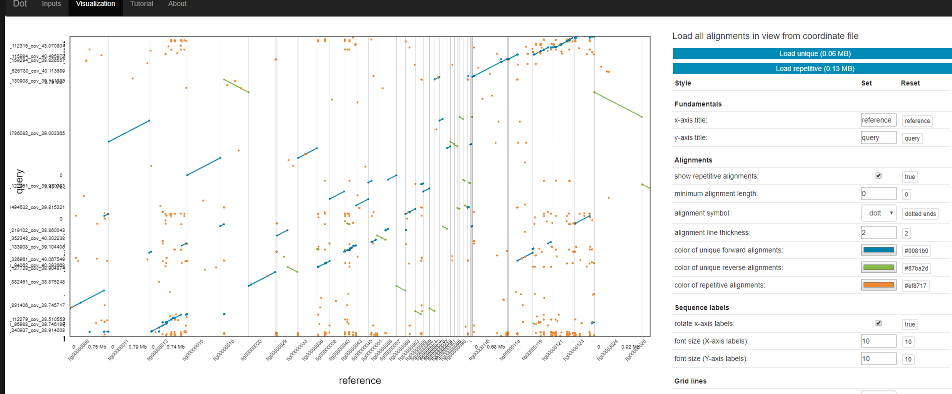
The output of DotPrep.py includes the *.coords and *.coords.idx that should be used with Dot for visualization.
Which one is the best?
BUSCO
BUSCO assessments are implemented in open-source software, with a large selection of lineage-specific sets of Benchmarking Universal Single-Copy Orthologs. These conserved orthologs are ideal candidates for large-scale phylogenomics studies, and the annotated BUSCO gene models built during genome assessments provide a comprehensive gene predictor training set for use as part of genome annotation pipelines.
https://busco.ezlab.org/
cd /data/gpfs/assoc/bch709-1/<YOURID>/Genome_assembly/
mkdir BUSCO
cd BUSCO
cp /data/gpfs/assoc/bch709-1/<YOURID>/Genome_assembly/genomeassembly_results/*.fasta .
 cp /data/gpfs/assoc/bch709-1/<YOURID>/Genome_assembly/Pilon/canu.illumina.fasta .

conda create -n busco4  python=3.6
conda activate busco4
conda install -c bioconda -c conda-forge busco=4.0.5 multiqc=1.9 biopython
Create job file
nano busco.sh
busco -l viridiplantae_odb10 --cpu 24 --in spades_illumina.fasta --out BUSCO_Illumina --mode genome  -f

busco -l viridiplantae_odb10 --cpu 24 --in spades_pacbio_illumina.fasta --out BUSCO_Illumina_Pacbio --mode genome  -f

busco -l viridiplantae_odb10 --cpu 24 --in canu.contigs.fasta   --out BUSCO_Pacbio --mode genome  -f

busco -l viridiplantae_odb10 --cpu 24 --in canu.illumina.fasta   --out BUSCO_Pacbio_Pilon --mode genome  -f

multiqc . -n assembly
Execute
chmod 775 busco.sh
./busco.sh
BUSCO results
INFO:   Results:        C:10.8%[S:10.8%,D:0.0%],F:0.5%,M:88.7%,n:425

INFO:

        --------------------------------------------------
        |Results from dataset viridiplantae_odb10         |
        --------------------------------------------------
        |C:10.8%[S:10.8%,D:0.0%],F:0.5%,M:88.7%,n:425     |
        |46     Complete BUSCOs (C)                       |
        |46     Complete and single-copy BUSCOs (S)       |
        |0      Complete and duplicated BUSCOs (D)        |
        |2      Fragmented BUSCOs (F)                     |
        |377    Missing BUSCOs (M)                        |
        |425    Total BUSCO groups searched               |
        --------------------------------------------------
INFO:   BUSCO analysis done. Total running time: 123 seconds
mkdir BUSCO_result
cp BUSCO_*/*.txt BUSCO_result
generate_plot.py -wd BUSCO_result
Assignment
Please generate report by MultiQC and upload your results to WebCampus.
Genome Annotation
Conda environment
Please use all lower case this time
conda deactivate
conda create -n genomeannotation  -y
conda activate genomeannotation
conda install -c bioconda -c conda-forge augustus=3.3.3 maker  repeatmasker snap  -y
conda install -c bioconda -c conda-forge -c anaconda rmblast -y
After the sections of DNA sequence have been assembled into a complete genome sequence we need to identify where the genes and key features are. We have our aligned and assembled genome sequence but how do we identify where the genes and other functional regions of the genome are located.
-
Annotation involves marking where the genes start and stop in the DNA sequence and also where other relevant and interesting regions are in the sequence.
-
Although genome annotation pipelines can differ from one another, for example, some elements can be manual while others have to be automated, they all share a core set of features.
-
They are generally divided into two distinct phases: gene prediction and manual annotation.
Gene prediction
There are two types of gene prediction: Ab initio – this technique relies on signals within the DNA sequence. It is an automated process whereby a computer is given instructions for finding genes in the sequence and is then left to find them. The computer looks for common sequences known to be found at the start and end of genes such as promoter sequences (where proteins bind that switch on genes), start codons (where the code for the gene product, RNA ?or protein, starts) and stop codons (where the code for the gene product ends).
Evidence-based
This technique relies on evidence beyond the DNA sequence. It involves gathering various pieces of genetic information from the transcript sequence (mRNA), and known protein sequences of the genome. With these pieces of evidence it is then possible to get an idea of the original DNA sequence by working backwards through transcription? and translation? (reverse transcription/translation). For example, if you have the protein sequence it is possible to work out the family of possible DNA sequences it could be derived from by working out which amino acids? make up the protein and then which combination of codons could code for those amino acids and so on, until you get to the DNA sequence. The information taken from these two prediction methods is then combined and lined up with the sequenced genome.
Key Point
-
Gene annotation is one of the core mechanisms through which we decipher the information that is contained in genome sequences.
-
Gene annotation is complicated by the existence of ‘transcriptional complexity’, which includes extensive alternative splicing and transcriptional events outside of protein-coding genes.
-
The annotation strategy for a given genome will depend on what it is hoped to achieve, as well as the resources available.
-
The availability of next-generation data sets has transformed gene annotation pipelines in recent years, although their incorporation is rarely straightforward.
-
Even human gene annotation is far from complete: transcripts are missing and existing models are truncated. Most importantly, ‘functional annotation’ — the description of what transcripts actually do — remains far from comprehensive.
-
Efforts are now under way to integrate gene annotation pipelines with projects that seek to describe regulatory sequences, such as promoter and enhancer elements.
-
Gene annotation is producing increasingly complex resources. This can present a challenge to usability, most notably in a clinical context, and annotation projects must find ways to resolve such problems.
The core annotation workflows for different gene types.
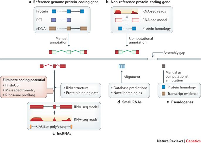
| These workflows illustrate general annotation principles rather than the specific pipelines of any particular genebuild. a | Protein-coding genes within reference genomes were generally annotated on the basis of the computational genomic alignment of Sanger-sequenced transcripts and protein-coding sequences, followed by manual annotation using interface tools such as Zmap, WebApollo, Artemis and the Integrative Genomics Viewer. Transcripts were typically taken from GenBank129 and proteins from Swiss-Prot. b | Protein-coding genes within non-reference genomes are usually annotated based on fewer resources; in this case, RNA sequencing (RNA-seq) data are used in combination with protein homology information that has been extrapolated from a closely related genome. RNA-seq pipelines for read alignment include STAR and TopHat, whereas model creation is commonly carried out by Cufflinks23. c | Long non-coding RNA (lncRNA) structures can be annotated in a similar manner to protein-coding transcripts (parts a and b), although coding potential must be ruled out. This is typically done by examining sequence conservation with PhyloCSF or using experimental data sets, such as mass spectrometry or ribosome profiling. In this example, 5′ Cap Analysis of Gene Expression (CAGE) and polyA-seq data are also incorporated to obtain true transcript end points. Designated lncRNA pipelines include PLAR. d | Small RNAs are typically added to genebuilds by mining repositories such as RFAM or miRBase. However, these entries can be used to search for additional loci based on homology. e | Pseudogene annotation is based on the identification of loci with protein homology to either paralogous or orthologous protein-coding genes. Computational annotation pipelines include PseudoPipe53, although manual annotation is more accurate. Finally, all annotation methods can be thwarted by the existence of sequence gaps in the genome assembly (right-angled arrow). EST, expressed sequence tag. |
High-level strategies for gene annotation projects.
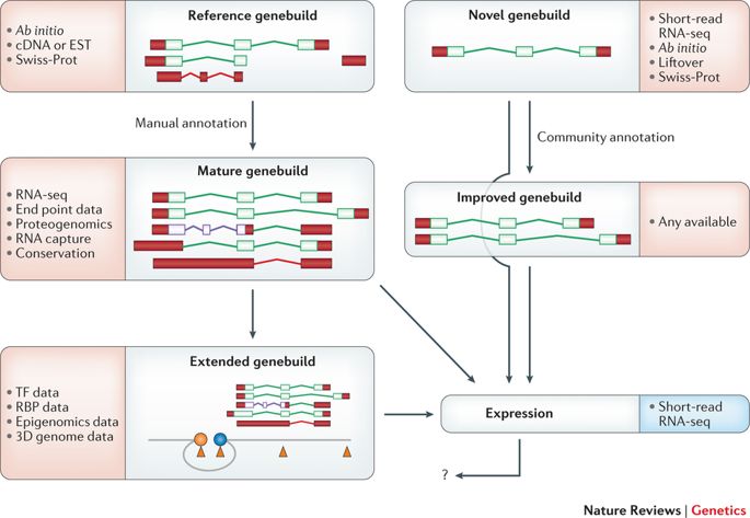
This schematic details the annotation pathways for reference and novel genomes. Coding sequences (CDSs) are outlined in green, nonsense-mediated decay (NMD) is shown in purple and untranslated regions (UTRs) are filled in in red. The core evidence sets that are used at each stage are listed, although their availability and incorporation can vary across different projects. The types of evidence used for reference genebuilds have evolved over time: RNA sequencing (RNA-seq) has replaced Sanger sequencing, conservation-based methodologies have become more powerful and proteogenomic data sets are now available. By contrast, novel genebuilds are constructed based on RNA-seq and/or ab initio modelling, in combination with the projection of annotation from other species (which is known as liftover) and the use of other species evidence sets. In fact, certain novel genebuilds such as those of pigs and rats now incorporate a modest amount of manual annotation, and could perhaps be described as ‘intermediate’ in status between ‘novel’ and ‘reference’. Furthermore, such genebuilds have also been improved by community annotation; this process typically follows the manual annotation workflows for reference genomes, although on a smaller scale. Although all reference genebuilds are ‘mature’ in our view, progress into the ‘extended genebuild’ phase is most advanced for humans. A promoter is indicated by the blue circle, an enhancer is indicated by the orange circle, and binding sites for transcription factors (TFs) or RNA-binding proteins (RBPs) are shown as orange triangles. Gene expression can be analysed on any genebuild regardless of quality, although it is more effective when applied to accurate transcript catalogues. Clearly, the results of expression analyses have the potential to reciprocally improve the efficacy of genebuilds, although it remains to be seen how this will be achieved in practice (indicated by the question mark). 3D, three-dimensional; EST, expressed sequence tag.
General Considerations
Bacteria use ATG as their main start codon, but GTG and TTG are also fairly common, and a few others are occasionally used.
– Remember that start codons are also used internally: the actual start codon may not be the first one in the ORF.
Please check Genetic code
The stop codons are the same as in eukaryotes: TGA, TAA, TAG
– stop codons are (almost) absolute: except for a few cases of programmed frameshifts and the use of TGA for selenocysteine, the stop codon at the end of an ORF is the end of protein translation.
Genes can overlap by a small amount. Not much, but a few codons of overlap is common enough so that you can’t just eliminate overlaps as impossible.
- Cross-species homology works well for many genes. It is very unlikely that noncoding sequence will be conserved. – But, a significant minority of genes (say 20%) are unique to a given species.
Translation start signals (ribosome binding sites; Shine-Dalgarno sequences) are often found just upstream from the start codon
– however, some aren’t recognizable – genes in operons sometimes don’t always have a separate ribosome binding site for each gene
Based on hidden Markov model (HMM)
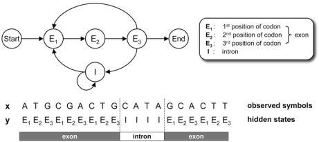
- As you move along the DNA sequence, a given nucleotide can be in an exon or an intron or in an intergenic region.
- The oversimplified model on this slide doesn’t have the ”non-gene” state
- Use a training set of known genes (from the same or closely related species) to determine transmission and emission probabilities.
Very simple HMM: each base is either in an intron or an exon, and gets emitted with different frequencies depending on which state it is in.
A simple HMM for modeling eukaryotic genes.
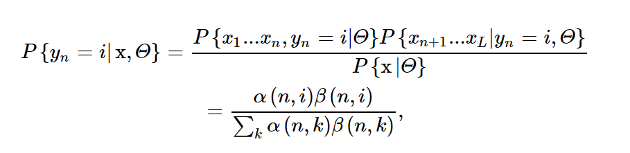
| The posterior probability P{yn = i | x, Θ} can be computed from |
Genome Annotation
mkdir /data/gpfs/assoc/bch709-1/<YOURID>/tmp

mkdir /data/gpfs/assoc/bch709-1/<YOURID>/genomeannotation

cd !$
Conda environment
Please use all lower case this time
conda create -n genomeannotation -y
conda activate genomeannotation
conda install -c bioconda -c conda-forge augustus=3.3.3 maker  repeatmasker snap  -y
conda install -c bioconda -c conda-forge -c anaconda rmblast -y
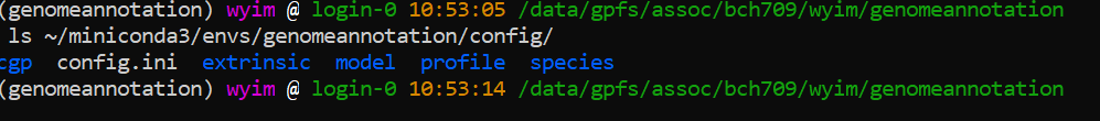
Setting augustus
ls ~/miniconda3/envs/genomeannotation/config/
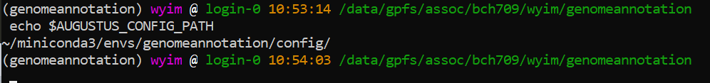
export AUGUSTUS_CONFIG_PATH=/data/gpfs/home/<YOURID>/miniconda3/envs/genomeannotation/config/
echo $AUGUSTUS_CONFIG_PATH
ls $AUGUSTUS_CONFIG_PATH
If there’s an error, please check typo first
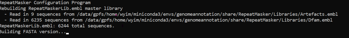
Setting RepeatMaker
cd ~/miniconda3/envs/genomeannotation/share/RepeatMasker
./configure
PUSH ENTER
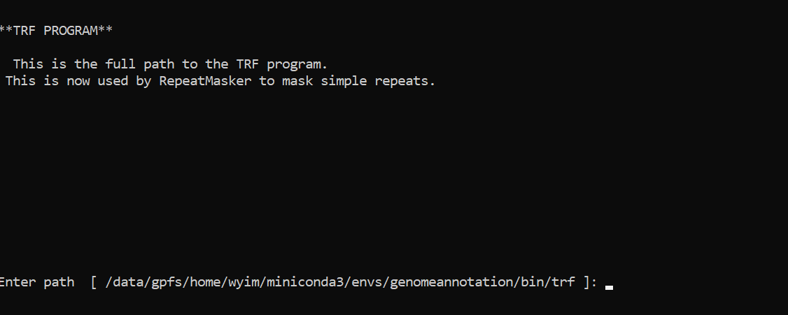
type 2
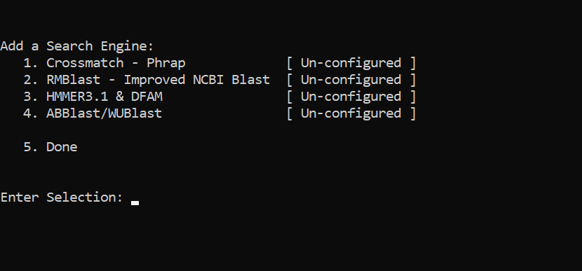
/data/gpfs/home/YOURID/miniconda3/envs/genomeannotation/bin/
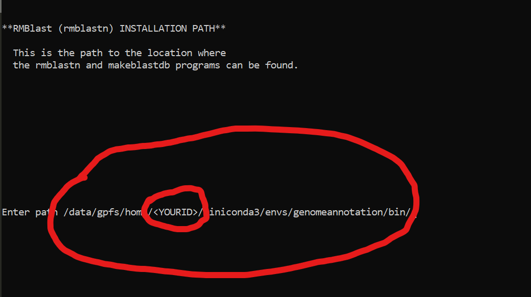
type Y
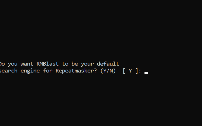
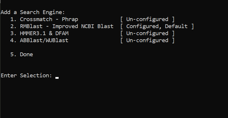
type 5
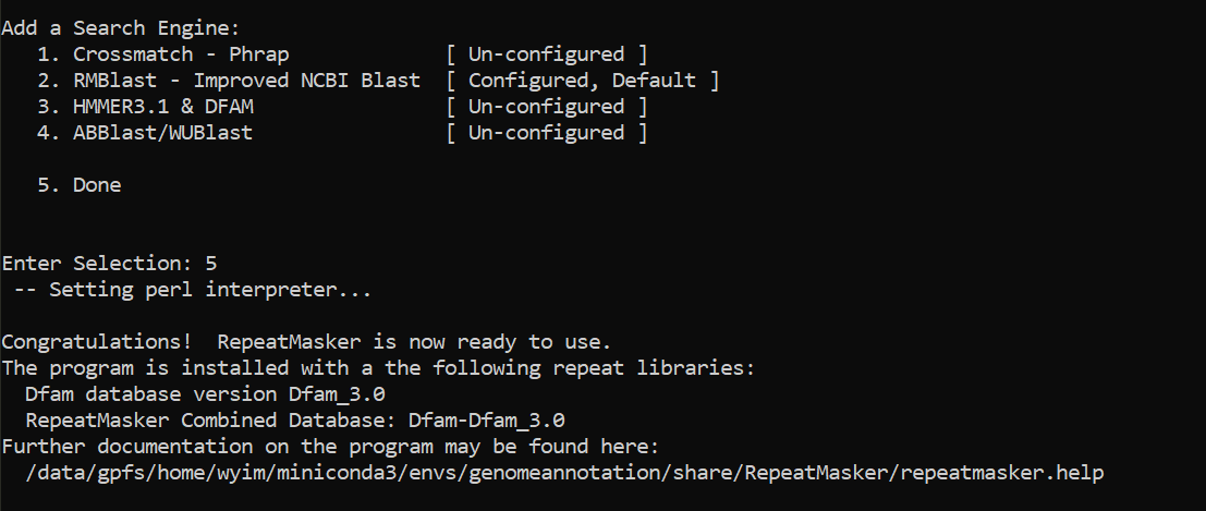
cd -
Copy your draft genome
wget https://www.dropbox.com/s/xpnhj6j99dr1kum/Athaliana_subset_BCH709.fa
cp Athaliana_subset_BCH709.fa bch709_assembly.fasta
MAKER software
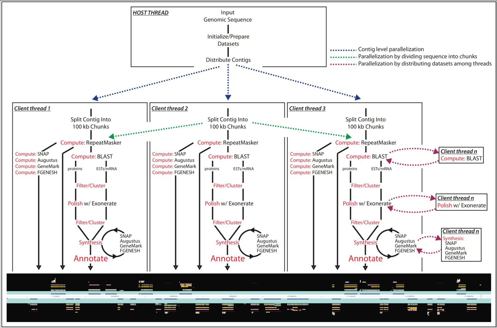
MAKER is a portable and easily configurable genome annotation pipeline. Its purpose is to allow smaller eukaryotic and prokaryotic genome projects to independently annotate their genomes and to create genome databases. MAKER identifies repeats, aligns ESTs and proteins to a genome, produces ab-initio gene predictions and automatically synthesizes these data into gene annotations having evidence-based quality values. MAKER is also easily trainable: outputs of preliminary runs can be used to automatically retrain its gene prediction algorithm, producing higher quality gene-models on seusequent runs. MAKER’s inputs are minimal and its ouputs can be directly loaded into a GMOD database. They can also be viewed in the Apollo genome browser; this feature of MAKER provides an easy means to annotate, view and edit individual contigs and BACs without the overhead of a database. MAKER should prove especially useful for emerging model organism projects with minimal bioinformatics expertise and computer resources.
Test MAKER
maker --help
Generate Control files
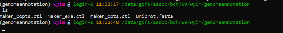
maker -CTL
This is normal

ls
Update Control files with below options
nano maker_opts.ctl
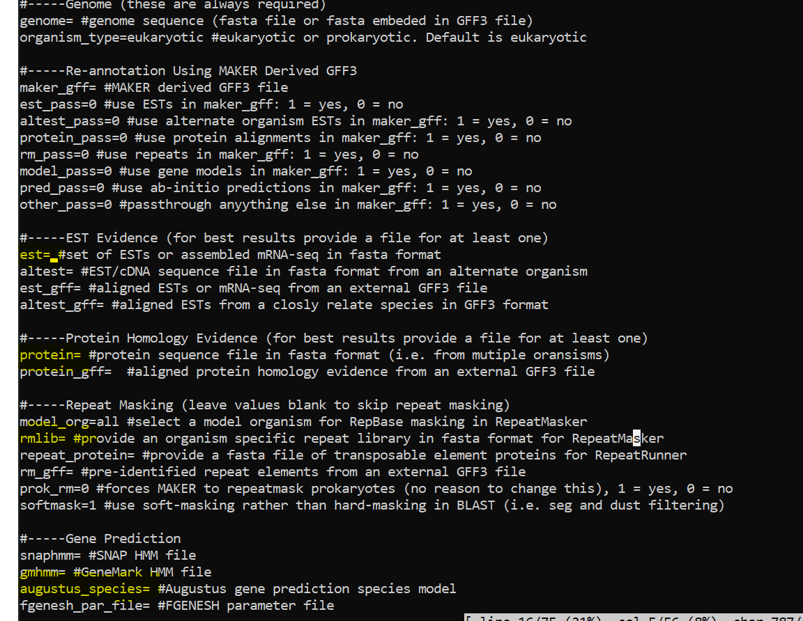
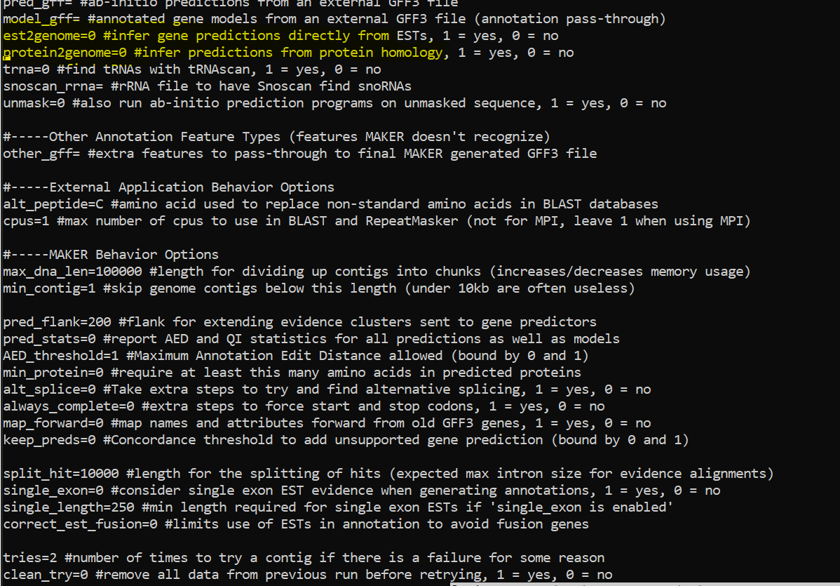

Update control file example
Update below
est=/data/gpfs/assoc/bch709-1/Course_material/maker/Trinity.fasta
rmlib=/data/gpfs/assoc/bch709-1/Course_material/maker/te_proteins.fasta
protein=/data/gpfs/assoc/bch709-1/Course_material/maker/uniprot_sprot.fasta
augustus_species=arabidopsis
est2genome=1
protein2genome=1
TMP=/data/gpfs/assoc/bch709-1/<YOURID>/tmp  #YOURID
Run Maker
nano maker.sh
#!/bin/bash
#SBATCH --job-name=maker
#SBATCH --cpus-per-task=24
#SBATCH --time=7-12:00:00
#SBATCH --mem=20g
#SBATCH --mail-type=all
#SBATCH --mail-user=wyim@unr.edu
#SBATCH -o maker.out # STDOUT
#SBATCH -e maker.err # STDERR
#SBATCH -p cpu-s2-core-0
#SBATCH -A cpu-s2-bch709-1
export AUGUSTUS_CONFIG_PATH="~/miniconda3/envs/genomeannotation/config/"

maker -cpus 24 -base bch709  -genome bch709_assembly.fasta -fix_nucleotides
Genome annotation Results
cd /data/gpfs/assoc/bch709-1/<YOURID>/genomeannotation/bch709.maker.output

cat maker.err
 fasta_merge


Synopsis:

fasta_merge -d maker_datastore_index.log
fasta_merge -o genome.all -i <fasta1> <fasta2> ...

Descriptions:

This script will take a MAKER datastore index log file, extract all
the relevant fasta files and create fasta files with relevant
categories of sequence (i.e. transcript, protein, GeneMark protien,
etc.).  For this to work properly you need to be in the same directory
as the datastore index.

Options:

  -d The location of the MAKER datastore index log.
  -o Alternate base name for the output files.
  -i A optional list of files to process along with or instead of the
     datastore.
gff3_merge


Synopsis:

gff3_merge -d maker_datastore_index.log
gff3_merge -o genome.all.gff <gff3_file1> <gff3_file2> ...

Descriptions:

This script will take a MAKER datastore index log file, extract all
the relevant GFF3 files and combined GFF3 file.  The script can also
combine other correctly formated GFF3 files.  For this to work
properly you need to be in the same directory as the datastore index.

Options:

  -d The location of the MAKER datastore index log file.
  -o Alternate base name for the output files.
  -s Use STDOUT for output.
  -g Only write MAKER gene models to the file, and ignore evidence.
  -n Do not print fasta sequence in footer
  -l Merge legacy annotation sets (ignores already having seen
     features more than once for the same contig)
fasta_merge -d bch709.maker.output/bch709_master_datastore_index.log

gff3_merge -d bch709.maker.output/bch709_master_datastore_index.log -n -o bch709_all.gff

gff3_merge -d bch709.maker.output/bch709_master_datastore_index.log -n -g -o bch709.gff
GFF3 File Format - Definition and supported options
The GFF (General Feature Format) format consists of one line per feature, each containing 9 columns of data, plus optional track definition line. Fields The first line of a GFF3 file must be a comment that identifies the version, e.g.
##gff-version 3 Fields must be tab-separated. Also, all but the final field in each feature line must contain a value; “empty” columns should be denoted with a ‘.’
- seqid - name of the chromosome or scaffold; chromosome names can be given with or without the ‘chr’ prefix. Important note: the seq ID must be one used within Ensembl, i.e. a standard chromosome name or an Ensembl identifier such as a scaffold ID, without any additional content such as species or assembly. See the example GFF output below.
- source - name of the program that generated this feature, or the data source (database or project name)
- type - type of feature. Must be a term or accession from the SOFA sequence ontology
- start - Start position of the feature, with sequence numbering starting at 1.
- end - End position of the feature, with sequence numbering starting at 1.
- score - A floating point value.
- strand - defined as + (forward) or - (reverse).
- phase - One of ‘0’, ‘1’ or ‘2’. ‘0’ indicates that the first base of the feature is the first base of a codon, ‘1’ that the second base is the first base of a codon, and so on..
- attributes - A semicolon-separated list of tag-value pairs, providing additional information about each feature. Some of these tags are predefined, e.g. ID, Name, Alias, Parent - see the GFF documentation for more details.
Note that where the attributes contain Parent identifiers, these will be used by Ensembl to display the features as joined blocks.
Structure is as GFF, so the fields are:
<seqname> <source> <feature> <start> <end> <score> <strand> <frame> [attributes] [comments]
QI
- Length of the 5 UTR
- Fraction of splice sites confirmed by an EST alignment
- Fraction of exons that overlap an EST alignment
- Fraction of exons that overlap EST or Protein alignments
- Fraction of splice sites confirmed by a SNAP prediction
- Fraction of exons that overlap a SNAP prediction
- Number of exons in the mRNA
- Length of the 3 UTR
- Length of the protein sequence produced by the mRNA
Annotation Edit Distance (AED)
eAED is the the AED edit distance at an exon level, not base pair level like normal AED