RNA-Seq reads Count Analysis
pwd
### Your current location is
## /data/gpfs/assoc/bch709/<YOUR_ID>/rnaseq/DEG

nano <JOBNAME>.sh
RNA-Seq reads Count Analysis job script
#!/bin/bash
#SBATCH --job-name=<JOBNAME>
#SBATCH --cpus-per-task=16
#SBATCH --time=2:00:00
#SBATCH --mem=16g
#SBATCH --mail-type=begin
#SBATCH --mail-type=end
#SBATCH --mail-user=<YOUR ID>@unr.edu
#SBATCH -o <JOBNAME>.out # STDOUT
#SBATCH -e <JOBNAME>.err # STDERR

align_and_estimate_abundance.pl --transcripts Trinity.fasta --seqType fq --left /data/gpfs/assoc/bch709/<YOUR_NAME>/rnaseq/rawdata_rnaseq/fastq/pair1.fastq.gz --right /data/gpfs/assoc/bch709/<YOUR_NAME>/rnaseq/rawdata_rnaseq/fastq/pair2.fastq.gz  --est_method RSEM --aln_method bowtie2 --trinity_mode --prep_reference --output_dir rsem_outdir  --thread_count  16
Job submission
sbatch <JOBNAME>.sh
Job check
squeue
Job running check
## do ```ls``` first
ls

cat <YOUR_JOB>.err

cat <YOUR_JOB>.out

or

cat slurm_<JOBID>.out
RSEM results check
less rsem_outdir/RSEM.genes.results
Your current location is* /data/gpfs/assoc/bch709/spiderman/rnaseq/DEG
FPKM
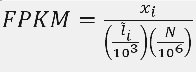
X = mapped reads count N = number of reads L = Length of transcripts
head -n 2 rsem_outdir/RSEM.genes.results
Reads count
samtools flagstat rsem_outdir/bowtie2.bam
Call Python
python
X = 861
Number_Reads_mapped = 1485483
Length = 3475
fpkm= X*(1000/Length)*(1000000/Number_Reads_mapped)
fpkm
ten to the ninth power = 10**9
fpkm=X/(Number_Reads_mapped*Length)*10**9
fpkm
FPKM
Fragments per Kilobase of transcript per million mapped reads
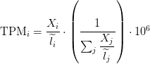
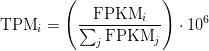
TPM
Transcripts Per Million
Sum of FPKM
cat rsem_outdir/RSEM.genes.results | egrep -v FPKM | awk '{ sum+=$7} END {print sum}'
TPM calculation from FPKM
FPKM = 180.61
SUM_FPKM = 646089
TPM=(FPKM/SUM_FPKM)*10**6
TPM
TPM calculation from reads count
cat rsem_outdir/RSEM.genes.results | egrep -v FPKM | awk '{ sum+=$5/$3} END {print sum}'
sum_count_per_length = 714.037

TPM = (X/Length)*(1/sum_count_per_length )*10**6
Paper read
Li et al., 2010, RSEM Dillies et al., 2013
Home work solve
File download
$ mkdir -p /data/gpfs/assoc/bch709/<YOUR_NAME>/rnaseq/homework2

$ cd /data/gpfs/assoc/bch709/<YOUR_NAME>/rnaseq/homework2
Download below files
mkdir fastq
cd fastq
pwd
#current directory should be /data/gpfs/assoc/bch709/<YOUR_NAME>/rnaseq/homework/fastq
- use
wgethttps://www.dropbox.com/s/mzvempzve7uuwoa/KRWTD1_1.fastq.gz https://www.dropbox.com/s/uv2a10w9wj9tcww/KRWTD1_2.fastq.gz https://www.dropbox.com/s/ra0s10g2nag6axp/KRWTD2_1.fastq.gz https://www.dropbox.com/s/jao5tb8a1hnzqw4/KRWTD2_2.fastq.gz https://www.dropbox.com/s/4gwhz0t1d32cdnw/KRWTD3_1.fastq.gz https://www.dropbox.com/s/wp2uk0nafdb74wp/KRWTD3_2.fastq.gz https://www.dropbox.com/s/ctzo9k9n8qdpvio/KRWTW1_1.fastq.gz https://www.dropbox.com/s/psiak4r2910sjsc/KRWTW1_2.fastq.gz https://www.dropbox.com/s/so4zeuyqz64m80z/KRWTW2_1.fastq.gz https://www.dropbox.com/s/2ggf2xdiydtehdw/KRWTW2_2.fastq.gz https://www.dropbox.com/s/7bfgcq69cymb5yj/KRWTW3_1.fastq.gz https://www.dropbox.com/s/lfif4qnbhnfes26/KRWTW3_2.fastq.gz
Run trimming
$ cd /data/gpfs/assoc/bch709/<YOUR_NAME>/rnaseq/homework2/fastq
$ nano <JOB_NAME>.sh
Submit trimming job with following criteria
- SBATCH
--time=2:00:00 --cpus-per-task=16 --mem-per-cpu=10g - trim_galore
trim_galore --paired --three_prime_clip_R1 20 --three_prime_clip_R2 20 --cores 16 --max_n 40 --gzip -o /data/gpfs/assoc/bch709/<YOUR_NAME>/rnaseq/homework/trim
Mock SBATCH example is below
#!/bin/bash
#SBATCH --job-name=<JOB_NAME>
#SBATCH --cpus-per-task=1
#SBATCH --time=2:00:00
#SBATCH --mem-per-cpu=1g
#SBATCH --mail-type=begin
#SBATCH --mail-type=end
#SBATCH --mail-user=<YOUR ID>@unr.edu


trim_galore --paired   --three_prime_clip_R1 20 --three_prime_clip_R2 20 --cores 16  --max_n 40  --gzip -o  /data/gpfs/assoc/bch709/<YOUR_NAME>/rnaseq/homework/trim /data/gpfs/assoc/bch709/<YOUR_NAME>/rnaseq/homework/fastq/KRWTD1_1.fastq.gz /data/gpfs/assoc/bch709/<YOUR_NAME>/rnaseq/homework/fastq/KRWTD1_2.fastq.gz
Job submission Requirement
chmod 775 <JOB_NAME>.sh
sbatch <JOB_NAME>.sh
Need to do all of samples
KRWTD1_1.fastq.gz KRWTD1_2.fastq.gz
KRWTD2_1.fastq.gz KRWTD2_2.fastq.gz
KRWTD3_1.fastq.gz KRWTD3_2.fastq.gz
KRWTW1_1.fastq.gz KRWTW1_2.fastq.gz
KRWTW2_1.fastq.gz KRWTW2_2.fastq.gz
KRWTW3_1.fastq.gz KRWTW3_2.fastq.gz
###Batch example for i in $(ls -1 .gz | sed ‘s/_.//g’ | sort -u); do echo $i;
Run FastQC on Pronghorn by using SBATCH
- SBATCH
--time=2:00:00 --cpus-per-task=16 --mem-per-cpu=10g - fastqc
You can do everything at once.
fastqc /data/gpfs/assoc/bch709/<YOUR_NAME>/rnaseq/homework/trim/*.gz
fastqc /data/gpfs/assoc/bch709/<YOUR_NAME>/rnaseq/homework/fastq/*.gz
PLEASE CHECK YOUR MULTIQC
Merge gz file (Pair1 and Pair2)
cd /data/gpfs/assoc/bch709/<YOUR_NAME>/rnaseq/homework/trim
For example
zcat /data/gpfs/assoc/bch709/<YOUR_NAME>/rnaseq/homework/trim/*.1.fq.gz  >> merged_R1.fastq

zcat /data/gpfs/assoc/bch709/<YOUR_NAME>/rnaseq/homework/trim/*.2.fq.gz  >> merged_R2.fastq
Trinity run
mkdir /data/gpfs/assoc/bch709/<YOUR_NAME>/rnaseq/homework/Trinity
cd /data/gpfs/assoc/bch709/<YOUR_NAME>/rnaseq/homework/Trinity
Submit Trinity job with following criteria
#!/bin/bash
#SBATCH --job-name=<JOB_NAME>
#SBATCH --cpus-per-task=64
#SBATCH --time=2:00:00
#SBATCH --mem=100g
#SBATCH --mail-type=begin
#SBATCH --mail-type=end
#SBATCH --mail-user=<YOUR ID>@unr.edu
#SBATCH -o <JOB_NAME>.out # STDOUT
#SBATCH -e <JOB_NAME>.err # STDERR

Trinity --seqType fq  --CPU 64 --max_memory 100G --left <PAIR1_MERGED_FILE_LOCATION> --right <PAIR2_MERGED_FILE_LOCATION>
MultiQC
cd /data/gpfs/assoc/bch709/<YOUR_NAME>/rnaseq/homework/
multiqc . -n <YOUR_NAME> --exclude rsem --exclude gatk
Please send me the results
cd /data/gpfs/assoc/bch709/<YOUR_NAME>/rnaseq/homework/Trinity/

egrep -c ">" trinity_out_dir/Trinity.fasta >> <YOUR_NAME>.trinity.stat

TrinityStats.pl trinity_out_dir/Trinity.fasta >> <YOUR_NAME>.trinity.stat
Use SCP for downloading and send me the file
***
** When you have an ERROR, please send me your history. “histoty » myhistory.txt” **
Activating Enviroment
conda activate rnaseq
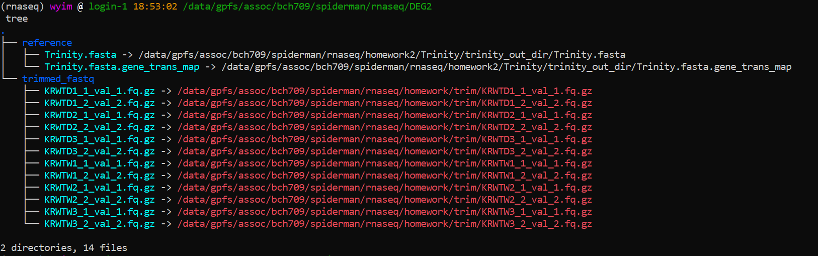
Starting Alignment
cd /data/gpfs/assoc/bch709/<YOUR_ID>/rnaseq/

mkdir DEG2

## move to DEG2 folder
cd DEG2

## Making folder
mkdir trimmed_fastq
mkdir reference

## Change Directory
cd trimmed_fastq

## link files
ln -s /data/gpfs/assoc/bch709/spiderman/rnaseq/homework/trim/*.gz .
ls -algh
zcat  KRWTD1_1_val_1.fq.gz | head

## Change Directory
cd ../
## Your directory should be /data/gpfs/assoc/bch709/spiderman/rnaseq/DEG2/

## Link reference
cd reference

ln -s  /data/gpfs/assoc/bch709/spiderman/rnaseq/homework/Trinity/trinity_out_dir/Trinity.fasta.gene_trans_map .

ln -s  /data/gpfs/assoc/bch709/spiderman/rnaseq/homework/Trinity/trinity_out_dir/Trinity.fasta .
Type sample file
conda install nano

nano sample.txt

###^ means CTRL key
###M- means ALT key
WT<TAB>WT_REP1<TAB>trimmed_fastq/KRWTW1_1_val_1.fq.gz<TAB>trimmed_fastq/KRWTW1_2_val_2.fq.gz
WT<TAB>WT_REP2<TAB>trimmed_fastq/KRWTW2_1_val_1.fq.gz<TAB>trimmed_fastq/KRWTW2_2_val_2.fq.gz
WT<TAB>WT_REP3<TAB>trimmed_fastq/KRWTW3_1_val_1.fq.gz<TAB>trimmed_fastq/KRWTW3_2_val_2.fq.gz
DT<TAB>DT_REP1<TAB>trimmed_fastq/KRWTD1_1_val_1.fq.gz<TAB>trimmed_fastq/KRWTD1_2_val_2.fq.gz
DT<TAB>DT_REP2<TAB>trimmed_fastq/KRWTD2_1_val_1.fq.gz<TAB>trimmed_fastq/KRWTD2_2_val_2.fq.gz
DT<TAB>DT_REP3<TAB>trimmed_fastq/KRWTD3_1_val_1.fq.gz<TAB>trimmed_fastq/KRWTD3_2_val_2.fq.gz
Run alignment
#!/bin/bash
#SBATCH --job-name=<JOB_NAME>
#SBATCH --cpus-per-task=32
#SBATCH --time=2:00:00
#SBATCH --mem=64g
#SBATCH --mail-type=begin
#SBATCH --mail-type=end
#SBATCH --mail-user=<YOUR ID>@nevada.unr.edu
#SBATCH -o <JOB_NAME>.out # STDOUT
#SBATCH -e <JOB_NAME>.err # STDERR

align_and_estimate_abundance.pl --thread_count 32 --transcripts reference/Trinity.fasta --seqType fq  --est_method RSEM --aln_method bowtie2  --trinity_mode --prep_reference --output_dir rsem_outdir --samples_file sample.txt
Install R-packages
conda install -c bioconda bioconductor-ctc bioconductor-deseq2 bioconductor-edger bioconductor-biobase bioconductor-qvalue r-ape r-gplots r-fastcluster
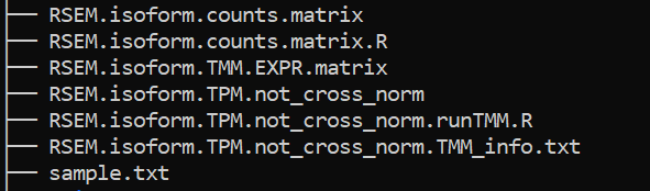
abundance_estimates_to_matrix
abundance_estimates_to_matrix.pl --est_method RSEM --gene_trans_map none --name_sample_by_basedir --cross_sample_norm TMM WT_REP1/RSEM.isoforms.results WT_REP2/RSEM.isoforms.results WT_REP3/RSEM.isoforms.results DT_REP1/RSEM.isoforms.results DT_REP2/RSEM.isoforms.results DT_REP3/RSEM.isoforms.results
Paper read
Li et al., 2010, RSEM Dillies et al., 2013
Normalization
CPM, RPKM, FPKM, TPM, RLE, MRN, Q, UQ, TMM, VST, RLOG, VOOM … Too many…
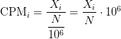
CPM: Controls for sequencing depth when dividing by total count. Not for within-sample comparison or DE.
Counts per million (CPM) mapped reads are counts scaled by the number of fragments you sequenced (N) times one million. This unit is related to the FPKM without length normalization and a factor of 10^3:
RPKM/FPKM: Controls for sequencing depth and gene length. Good for technical replicates, not good for sample-sample due to compositional bias. Assumes total RNA output is same in all samples. Not for DE.
TPM: Similar to RPKM/FPKM. Corrects for sequencing depth and gene length. Also comparable between samples but no correction for compositional bias.
TMM/RLE/MRN: Improved assumption: The output between samples for a core set only of genes is similar. Corrects for compositional bias. Used for DE. RLE and MRN are very similar and correlates well with sequencing depth. edgeR::calcNormFactors() implements TMM, TMMwzp, RLE & UQ. DESeq2::estimateSizeFactors implements median ratio method (RLE). Does not correct for gene length.
VST/RLOG/VOOM: Variance is stabilised across the range of mean values. For use in exploratory analyses. Not for DE. vst() and rlog() functions from DESeq2. voom() function from Limma converts data to normal distribution.
geTMM: Gene length corrected TMM.
For DGE using DGE R packages (DESeq2, edgeR, Limma etc), use raw counts
For visualisation (PCA, clustering, heatmaps etc), use TPM or TMM
For own analysis with gene length correction, use TPM (maybe geTMM?)
Other solutions: spike-ins/house-keeping genes
PtR (Quality Check Your Samples and Biological Replicates)
Once you’ve performed transcript quantification for each of your biological replicates, it’s good to examine the data to ensure that your biological replicates are well correlated, and also to investigate relationships among your samples. If there are any obvious discrepancies among your sample and replicate relationships such as due to accidental mis-labeling of sample replicates, or strong outliers or batch effects, you’ll want to identify them before proceeding to subsequent data analyses (such as differential expression).
cut -f 1,2 sample.txt >> samples_ptr.txt
PtR  --matrix RSEM.isoform.counts.matrix --samples samples_ptr.txt --CPM --log2 --min_rowSums 10  --compare_replicates

PtR  --matrix RSEM.isoform.counts.matrix --samples samples_ptr.txt --CPM  --log2 --min_rowSums 10   --sample_cor_matrix

PtR  --matrix RSEM.isoform.counts.matrix --samples samples_ptr.txt --CPM  --log2 --min_rowSums 10   --center_rows --prin_comp 3
Please transfer results to your local computer
DEG calculation
run_DE_analysis.pl --matrix RSEM.isoform.counts.matrix --samples_file samples_ptr.txt --method DESeq2
run_DE_analysis.pl --matrix RSEM.isoform.counts.matrix --samples_file samples_ptr.txt --method edgeR


cd DESeq2.XXXXX.dir
analyze_diff_expr.pl --matrix ../RSEM.isoform.TMM.EXPR.matrix  -P 0.001 -C 1  --samples ../samples_ptr.txt
wc -l RSEM.isoform.counts.matrix.DT_vs_WT.DESeq2.DE_results.P0.001_C1.DE.subset
cd ../

cd edgeR.XXXXX.dir
analyze_diff_expr.pl --matrix ../RSEM.isoform.TMM.EXPR.matrix  -P 0.001 -C 1  --samples ../samples_ptr.txt
wc -l RSEM.isoform.counts.matrix.DT_vs_WT.edgeR.DE_results.P0.001_C1.DE.subset
DESeq2 vs EdgeR Normalization method
DESeq and EdgeR are very similar and both assume that no genes are differentially expressed. DEseq uses a “geometric” normalisation strategy, whereas EdgeR is a weighted mean of log ratios-based method. Both normalise data initially via the calculation of size / normalisation factors.
Here is further information (important parts in bold):
DESeq
DESeq: This normalization method is included in the DESeq Bioconductor package (version 1.6.0) and is based on the hypothesis that most genes are not DE. A DESeq scaling factor for a given lane is computed as the median of the ratio, for each gene, of its read count over its geometric mean across all lanes. The underlying idea is that non-DE genes should have similar read counts across samples, leading to a ratio of 1. Assuming most genes are not DE, the median of this ratio for the lane provides an estimate of the correction factor that should be applied to all read counts of this lane to fulfill the hypothesis. By calling the estimateSizeFactors() and sizeFactors() functions in the DESeq Bioconductor package, this factor is computed for each lane, and raw read counts are divided by the factor associated with their sequencing lane.
DESeq2
EdgeR
Trimmed Mean of M-values (TMM): This normalization method is implemented in the edgeR Bioconductor package (version 2.4.0). It is also based on the hypothesis that most genes are not DE. The TMM factor is computed for each lane, with one lane being considered as a reference sample and the others as test samples. For each test sample, TMM is computed as the weighted mean of log ratios between this test and the reference, after exclusion of the most expressed genes and the genes with the largest log ratios. According to the hypothesis of low DE, this TMM should be close to 1. If it is not, its value provides an estimate of the correction factor that must be applied to the library sizes (and not the raw counts) in order to fulfill the hypothesis. The calcNormFactors() function in the edgeR Bioconductor package provides these scaling factors. To obtain normalized read counts, these normalization factors are re-scaled by the mean of the normalized library sizes. Normalized read counts are obtained by dividing raw read counts by these re-scaled normalization factors.
EdgeR
DESeq2 vs EdgeR Statistical tests for differential expression
DESeq2
DESeq2 uses raw counts, rather than normalized count data, and models the normalization to fit the counts within a Generalized Linear Model (GLM) of the negative binomial family with a logarithmic link. Statistical tests are then performed to assess differential expression, if any.
EdgeR
Data are normalized to account for sample size differences and variance among samples. The normalized count data are used to estimate per-gene fold changes and to perform statistical tests of whether each gene is likely to be differentially expressed.
EdgeR uses an exact test under a negative binomial distribution (Robinson and Smyth, 2008). The statistical test is related to Fisher’s exact test, though Fisher uses a different distribution.
Negative binormal
DESeq2
ϕ was assumed to be a function of μ determined by nonparametric regression. The recent version used in this paper follows a more versatile procedure. Firstly, for each transcript, an estimate of the dispersion is made, presumably using maximum likelihood. Secondly, the estimated dispersions for all transcripts are fitted to the functional form:
ϕ=a+bμ(DESeq parametric fit), using a gamma-family generalised linear model (Using regression)
EdgeR
edgeR recommends a “tagwise dispersion” function, which estimates the dispersion on a gene-by-gene basis, and implements an empirical Bayes strategy for squeezing the estimated dispersions towards the common dispersion. Under the default setting, the degree of squeezing is adjusted to suit the number of biological replicates within each condition: more biological replicates will need to borrow less information from the complete set of transcripts and require less squeezing.
Draw Venn Diagram
conda create -n venn python=2.7
conda activate venn
conda install -c bioconda bedtools intervene r-UpSetR=1.4.0 r-corrplot r-Cairo
cd ../
pwd
# /data/gpfs/assoc/bch709/spiderman/rnaseq/DEG2
mkdir Venn


###DESeq2
cut -f 1 ../DESeq2.91008.dir/RSEM.isoform.counts.matrix.DT_vs_WT.DESeq2.DE_results.P0.001_C1.DT-UP.subset  | grep -v sample > DESeq.UP.subset
cut -f 1 ../DESeq2.91008.dir/RSEM.isoform.counts.matrix.DT_vs_WT.DESeq2.DE_results.P0.001_C1.WT-UP.subset  | grep -v sample > DESeq.DOWN.subset

###edgeR
cut -f 1 ../edgeR.91693.dir/RSEM.isoform.counts.matrix.DT_vs_WT.edgeR.DE_results.P0.001_C1.DT-UP.subset   | grep -v sample > edgeR.UP.subset
cut -f 1 ../edgeR.91693.dir/RSEM.isoform.counts.matrix.DT_vs_WT.edgeR.DE_results.P0.001_C1.WT-UP.subset   | grep -v sample > edgeR.DOWN.subset


### Drawing
intervene venn -i DESeq.DOWN.subset DESeq.UP.subset edgeR.DOWN.subset edgeR.UP.subset  --type list --save-overlaps
intervene upset -i DESeq.DOWN.subset DESeq.UP.subset edgeR.DOWN.subset edgeR.UP.subset  --type list --save-overlaps
intervene pairwise  -i DESeq.DOWN.subset DESeq.UP.subset edgeR.DOWN.subset edgeR.UP.subset  --type list
Assignment
File download
$ mkdir -p /data/gpfs/assoc/bch709/<YOUR_NAME>/rnaseq/assignment1014

$ cd /data/gpfs/assoc/bch709/<YOUR_NAME>/rnaseq/assignment1014
Download below files
mkdir fastq
cd fastq
pwd
#current directory should be /data/gpfs/assoc/bch709/<YOUR_NAME>/rnaseq/homework/fastq
- use
wgethttps://www.dropbox.com/s/mcsy0kbcf0nike9/DT1_R1.fastq.gz https://www.dropbox.com/s/9qf82ln6unqjrcp/DT1_R2.fastq.gz https://www.dropbox.com/s/lua7zxh22xczdsv/DT2_R1.fastq.gz https://www.dropbox.com/s/cz0xzj5r6db199u/DT2_R2.fastq.gz https://www.dropbox.com/s/7rv4zy4wryniv97/DT3_R1.fastq.gz https://www.dropbox.com/s/sngak2gbrfdpzov/DT3_R2.fastq.gz https://www.dropbox.com/s/crjyoetliqizdaf/WT1_R1.fastq.gz https://www.dropbox.com/s/kdbj4dbp13kvumf/WT1_R2.fastq.gz https://www.dropbox.com/s/r1q2xpb3veuz8fc/WT2_R1.fastq.gz https://www.dropbox.com/s/i3c9up73z7pw1t0/WT2_R2.fastq.gz https://www.dropbox.com/s/a3jtfomg3m2jg40/WT3_R1.fastq.gz https://www.dropbox.com/s/opbupgn5zqox2x1/WT3_R2.fastq.gz
Run trimming
$ cd /data/gpfs/assoc/bch709/<YOUR_NAME>/rnaseq/assignment1014/fastq
$ nano <JOB_NAME>.sh
Submit trimming job with following criteria
- SBATCH
--time=2:00:00 --cpus-per-task=16 --mem-per-cpu=4g - trim_galore
trim_galore --paired --three_prime_clip_R1 20 --three_prime_clip_R2 20 --cores 16 --max_n 40 --gzip -o /data/gpfs/assoc/bch709/<YOUR_NAME>/rnaseq/assignment1014/trim
Mock SBATCH example is below
#!/bin/bash
#SBATCH --job-name=<JOB_NAME>
#SBATCH --cpus-per-task=16
#SBATCH --time=2:00:00
#SBATCH --mem-per-cpu=4g
#SBATCH --mail-type=begin
#SBATCH --mail-type=end
#SBATCH --mail-user=<YOUR ID>@unr.edu


trim_galore --paired   --three_prime_clip_R1 20 --three_prime_clip_R2 20 --cores 16  --max_n 40  --gzip -o  /data/gpfs/assoc/bch709/<YOUR_NAME>/rnaseq/homework/trim /data/gpfs/assoc/bch709/<YOUR_NAME>/rnaseq/assignment1014/fastq/WT1_R1.fastq.gz /data/gpfs/assoc/bch709/<YOUR_NAME>/rnaseq/assignment1014/fastq/WT1_R2.fastq.gz
Job submission Requirement
chmod 775 <JOB_NAME>.sh
sbatch <JOB_NAME>.sh
Need to do all of samples
DT1_R1.fastq.gz DT1_R2.fastq.gz
DT2_R1.fastq.gz DT2_R2.fastq.gz
DT3_R1.fastq.gz DT3_R2.fastq.gz
WT1_R1.fastq.gz WT1_R2.fastq.gz
WT2_R1.fastq.gz WT2_R2.fastq.gz
WT3_R1.fastq.gz WT3_R2.fastq.gz
fastqc
You can do everything at once.
fastqc
fastqc
Type sample file
nano sample.txt
Run alignment
align_and_estimate_abundance.pl
PtR (Quality Check Your Samples and Biological Replicates)
PtR
abundance_estimates_to_matrix
abundance_estimates_to_matrix.pl
DEG calculation by DESeq2
run_DE_analysis.pl

analyze_diff_expr.pl
Draw Venn Diagram
conda activate venn
intervene venn
MultiQC
cd /data/gpfs/assoc/bch709/<YOUR_NAME>/rnaseq/assignment1014/
multiqc . -n <YOUR_NAME> --exclude rsem --exclude gatk
PLEASE CHECK YOUR MULTIQC
Please send me the whole PDF results
DT.rep_compare
WT.rep_compare
RSEM.isoform.counts.matrix.minRow10.CPM.log2.centered.prcomp.principal_components
RSEM.isoform.counts.matrix.minRow10.log2.sample_cor_matrix
RSEM.isoform.counts.matrix.minRow10.CPM.log2.sample_cor_matrix
diffExpr.P0.001_C1.matrix.log2.centered.sample_cor_matrix.pdf
diffExpr.P0.001_C1.matrix.log2.centered.genes_vs_samples_heatmap.pdf
RSEM.isoform.counts.matrix.DT_vs_WT.DESeq2.DE_results.MA_n_Volcano.pdf
Intervene_venn.pdf
Office Hour
Fri Hackathon Mon 10am-noon