Trinity installation
conda env remove -n transcriptome_assembly -y

conda env update -n transcriptome_assembly --file /data/gpfs/assoc/bch709-4/Course_materials/transcriptome.yaml


conda activate transcriptome_assembly
Conda env
conda activate transcriptome_assembly
Create job submission script
cd /data/gpfs/assoc/bch709-4/${USER}/rnaseq_assembly/
nano trinity.sh
#!/bin/bash
#SBATCH --job-name="TRINITY"
#SBATCH --time=10:15:00
#SBATCH --account=cpu-s5-bch709-4
#SBATCH --partition=cpu-core-0
#SBATCH --cpus-per-task=8
#SBATCH --mem=80g
#SBATCH --mail-type=fail
#SBATCH --mail-type=begin
#SBATCH --mail-type=end
#SBATCH --mail-user=${USER}@unr.edu
#SBATCH --output=TRINITY.out


Trinity --seqType fq  --CPU 8 --max_memory 80G --left trim/DT1_R1_val_1.fq.gz,trim/DT2_R1_val_1.fq.gz,trim/DT3_R1_val_1.fq.gz,trim/WT1_R1_val_1.fq.gz,trim/WT2_R1_val_1.fq.gz,trim/WT3_R1_val_1.fq.gz --right trim/DT1_R2_val_2.fq.gz,trim/DT2_R2_val_2.fq.gz,trim/DT3_R2_val_2.fq.gz,trim/WT1_R2_val_2.fq.gz,trim/WT2_R2_val_2.fq.gz,trim/WT3_R2_val_2.fq.gz
Job submission
sbatch trinity.sh
Please check the result
cd /data/gpfs/assoc/bch709-4/${USER}/rnaseq_assembly

egrep -c ">"  trinity_out_dir.Trinity.fasta

TrinityStats.pl /data/gpfs/assoc/bch709-4/${USER}/rnaseq_assembly/trinity_out_dir.Trinity.fasta  > ${USER}.trinity.stat

cat ${USER}.trinity.stat
RNA-Seq reads Count Analysis
pwd
### Your current location is
## /data/gpfs/assoc/bch709-4/wyim/rnaseq_assembly
align_and_estimate_abundance.pl


nano reads_count.sh
JOBNAME and JOBID need to be changed
To check JOBID
squeue -u ${USER}
RNA-Seq reads Count Analysis job script
#!/bin/bash
#SBATCH --job-name=<JOBNAME>
#SBATCH --dependency=afterok:<JOBID>
#SBATCH -o <JOBNAME>.out # STDOUT
#SBATCH -e <JOBNAME>.err # STDERR
#SBATCH --mail-user=${USER}@unr.edu
#SBATCH --cpus-per-task=16
#SBATCH --time=15:00
#SBATCH --mem=16g
#SBATCH --mail-type=begin
#SBATCH --mail-type=end
#SBATCH --mail-type=fail
#SBATCH --account=cpu-s5-bch709-4
#SBATCH --partition=cpu-core-0


align_and_estimate_abundance.pl --transcripts trinity_out_dir.Trinity.fasta --seqType fq --left trim/DT1_R1_val_1.fq.gz --right trim/DT1_R2_val_2.fq.gz --est_method RSEM --aln_method bowtie2 --trinity_mode --prep_reference --output_dir rsem_outdir_test  --thread_count  16
Job submission
sbatch reads_count.sh
Job check
squeue -u ${USER}
Job running check
## do ```ls``` first
## CHANGE JOBNAME to your JOBNAME
ls
cat <JOBNAME>.out
cat <JOBNAME>.out
RSEM results check
less rsem_outdir_test/RSEM.genes.results
Expression values and Normalization
CPM, RPKM, FPKM, TPM, RLE, MRN, Q, UQ, TMM, VST, RLOG, VOOM … Too many…
CPM: Controls for sequencing depth when dividing by total count. Not for within-sample comparison or DE.
Counts per million (CPM) mapped reads are counts scaled by the number of fragments you sequenced (N) times one million. This unit is related to the FPKM without length normalization and a factor of 10^6:
RPKM/FPKM: Controls for sequencing depth and gene length. Good for technical replicates, not good for sample-sample due to compositional bias. Assumes total RNA output is same in all samples. Not for DE.
TPM: Similar to RPKM/FPKM. Corrects for sequencing depth and gene length. Also comparable between samples but no correction for compositional bias.
TMM/RLE/MRN: Improved assumption: The output between samples for a core set only of genes is similar. Corrects for compositional bias. Used for DE. RLE and MRN are very similar and correlates well with sequencing depth. edgeR::calcNormFactors() implements TMM, TMMwzp, RLE & UQ. DESeq2::estimateSizeFactors implements median ratio method (RLE). Does not correct for gene length.
VST/RLOG/VOOM: Variance is stabilised across the range of mean values. For use in exploratory analyses. Not for DE. vst() and rlog() functions from DESeq2. voom() function from Limma converts data to normal distribution.
geTMM: Gene length corrected TMM.
For DEG using DEG R packages (DESeq2, edgeR, Limma etc), use raw counts
For visualisation (PCA, clustering, heatmaps etc), use TPM or TMM
For own analysis with gene length correction, use TPM (maybe geTMM?)
Other solutions: spike-ins/house-keeping genes
FPKM
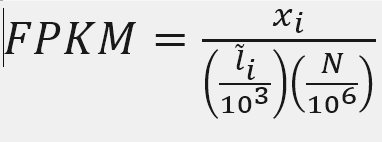
X = mapped reads count N = number of reads L = Length of transcripts
head -n 2 rsem_outdir_test/RSEM.genes.results
‘length’ is this transcript’s sequence length (poly(A) tail is not counted). ‘effective_length’ counts only the positions that can generate a valid fragment.
Reads count
samtools flagstat rsem_outdir_test/bowtie2.bam
less rsem_outdir_test/RSEM.genes.results
cat rsem_outdir_test/RSEM.genes.results | egrep -v FPKM | awk '{ sum+=$5} END {print sum}'
Call Python
python
FPKM
Fragments per Kilobase of transcript per million mapped reads
expectied_count = 14
Number_Reads_mapped =  1.4443e+06
Effective_Length = 1929.93
fpkm= expectied_count*(1000/Effective_Length)*(1000000/Number_Reads_mapped)
fpkm
ten to the ninth power = 10**9
fpkm=expectied_count/(Number_Reads_mapped*Effective_Length)*10**9
fpkm
TPM
Transcripts Per Million
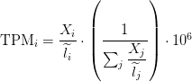
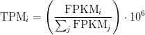
TPM calculation from reads count
cat rsem_outdir_test/RSEM.genes.results | egrep -v FPKM | awk '{ sum+=$5/$4} END {print sum}'
sum_count_per_length = 1169.65
expectied_count = 14
Effective_Length = 1929.93
TPM = (expectied_count/Effective_Length)*(1/sum_count_per_length )*10**6
TPM
TPM calculation from FPKM
Sum of FPKM
cat rsem_outdir_test/RSEM.genes.results | egrep -v FPKM | awk '{ sum+=$7} END {print sum}'
FPKM = 5.022605493468516
SUM_FPKM = 809843
TPM=(FPKM/SUM_FPKM)*10**6
TPM
Paper read
DEG calculation
Conda env
conda activate transcriptome_assembly
File prepare
cd /data/gpfs/assoc/bch709-4/${USER}/rnaseq_assembly/
Type sample file
nano sample.txt
###^ means CTRL key ###M- means ALT key
WT<TAB>WT_REP1<TAB>trim/WT1_R1_val_1.fq.gz<TAB>trim/WT1_R2_val_2.fq.gz
WT<TAB>WT_REP2<TAB>trim/WT2_R1_val_1.fq.gz<TAB>trim/WT2_R2_val_2.fq.gz
WT<TAB>WT_REP3<TAB>trim/WT3_R1_val_1.fq.gz<TAB>trim/WT3_R2_val_2.fq.gz
DT<TAB>DT_REP1<TAB>trim/DT1_R1_val_1.fq.gz<TAB>trim/DT1_R2_val_2.fq.gz
DT<TAB>DT_REP2<TAB>trim/DT2_R1_val_1.fq.gz<TAB>trim/DT2_R2_val_2.fq.gz
DT<TAB>DT_REP3<TAB>trim/DT3_R1_val_1.fq.gz<TAB>trim/DT3_R2_val_2.fq.gz
Change charater to Tab
sed 's/<TAB>/\t/g' sample.txt

sed -i 's/<TAB>/\t/g' sample.txt
Linux command explaination
https://explainshell.com/
https://explainshell.com/explain?cmd=cat+rsem_outdir_test%2FRSEM.genes.results+%7C+egrep+-v+FPKM+%7C+awk+%27%7B+sum%2B%3D%245%7D+END+%7Bprint+sum%7D%27#
SED AWK explaination
https://emb.carnegiescience.edu/sites/default/files/140602-sedawkbash.key_.pdf
Job file create
nano alignment.sh
JOBNAME and JOBID need to be changed
Run alignment
#!/bin/bash
#SBATCH --job-name=<JOBNAME>
#SBATCH --dependency=afterok:<JOBID>
#SBATCH -o <JOBNAME>.out # STDOUT
#SBATCH -e <JOBNAME>.err # STDERR
#SBATCH --mail-user=${USER}@unr.edu
#SBATCH --cpus-per-task=32
#SBATCH --time=1:15:00
#SBATCH --mem=64g
#SBATCH --mail-type=begin
#SBATCH --mail-type=end
#SBATCH --mail-type=fail
#SBATCH --mail-user=${USER}@nevada.unr.edu
#SBATCH --account=cpu-s5-bch709-4
#SBATCH --partition=cpu-core-0

align_and_estimate_abundance.pl --thread_count 32 --transcripts trinity_out_dir.Trinity.fasta --seqType fq  --est_method RSEM --aln_method bowtie2  --trinity_mode --prep_reference --samples_file sample.txt
abundance_estimates_to_matrix
mkdir DEG && cd DEG
nano abundance.sh
JOBNAME and JOBID need to be changed
#!/bin/bash
#SBATCH --job-name=<JOBNAME>
#SBATCH --dependency=afterok:<JOBID>
#SBATCH -o <JOBNAME>.out # STDOUT
#SBATCH -e <JOBNAME>.err # STDERR
#SBATCH --mail-user=${USER}@unr.edu
#SBATCH --cpus-per-task=1
#SBATCH --time=15:00
#SBATCH --mem=12g
#SBATCH --mail-type=begin
#SBATCH --mail-type=end
#SBATCH --mail-type=fail
#SBATCH --account=cpu-s5-bch709-4
#SBATCH --partition=cpu-core-0

abundance_estimates_to_matrix.pl  --est_method RSEM --gene_trans_map none --name_sample_by_basedir  --cross_sample_norm TMM ../WT_REP1/RSEM.isoforms.results ../WT_REP2/RSEM.isoforms.results ../WT_REP3/RSEM.isoforms.results   ../DT_REP1/RSEM.isoforms.results ../DT_REP2/RSEM.isoforms.results ../DT_REP3/RSEM.isoforms.results
sbatch abundance.sh
PtR (Quality Check Your Samples and Biological Replicates)
Once you’ve performed transcript quantification for each of your biological replicates, it’s good to examine the data to ensure that your biological replicates are well correlated, and also to investigate relationships among your samples. If there are any obvious discrepancies among your sample and replicate relationships such as due to accidental mis-labeling of sample replicates, or strong outliers or batch effects, you’ll want to identify them before proceeding to subsequent data analyses (such as differential expression).
cut -f 1,2 ../sample.txt >> samples_ptr.txt

nano ptr.sh
JOBNAME and JOBID need to be changed
#!/bin/bash
#SBATCH --job-name=<JOBNAME>
#SBATCH --dependency=afterok:<JOBID>
#SBATCH -o <JOBNAME>.out # STDOUT
#SBATCH -e <JOBNAME>.err # STDERR
#SBATCH --mail-user=${USER}@unr.edu
#SBATCH --cpus-per-task=1
#SBATCH --time=15:00
#SBATCH --mem=12g
#SBATCH --mail-type=begin
#SBATCH --mail-type=end
#SBATCH --mail-type=fail
#SBATCH --account=cpu-s5-bch709-4
#SBATCH --partition=cpu-core-0

PtR  --matrix RSEM.isoform.counts.matrix --samples samples_ptr.txt --CPM --log2 --min_rowSums 10  --compare_replicates

PtR  --matrix RSEM.isoform.counts.matrix --samples samples_ptr.txt --CPM  --log2 --min_rowSums 10   --sample_cor_matrix

PtR  --matrix RSEM.isoform.counts.matrix --samples samples_ptr.txt --CPM  --log2 --min_rowSums 10   --center_rows --prin_comp 3
Please transfer results to your local computer
DEG calculation
nano deseq.sh
JOBNAME and JOBID need to be changed
#!/bin/bash
#SBATCH --job-name=<JOBNAME>
#SBATCH --dependency=afterok:<JOBID>
#SBATCH -o <JOBNAME>.out # STDOUT
#SBATCH -e <JOBNAME>.err # STDERR
#SBATCH --mail-user=${USER}@unr.edu
#SBATCH --cpus-per-task=1
#SBATCH --time=15:00
#SBATCH --mem=12g
#SBATCH --mail-type=begin
#SBATCH --mail-type=end
#SBATCH --mail-type=fail
#SBATCH --account=cpu-s5-bch709-4
#SBATCH --partition=cpu-core-0


run_DE_analysis.pl --matrix RSEM.isoform.counts.matrix --samples_file samples_ptr.txt --method DESeq2
nano edgeR.sh
#!/bin/bash
#SBATCH --job-name=<JOB_NAME>
#SBATCH --cpus-per-task=1
#SBATCH --time=15:00
#SBATCH --mem=12g
#SBATCH --mail-type=begin
#SBATCH --mail-type=end
#SBATCH --mail-type=fail
#SBATCH --mail-user=${USER}@nevada.unr.edu
#SBATCH -o <JOB_NAME>.out # STDOUT
#SBATCH -e <JOB_NAME>.err # STDERR
#SBATCH --account=cpu-s5-bch709-4
#SBATCH --partition=cpu-core-0

run_DE_analysis.pl --matrix RSEM.isoform.counts.matrix --samples_file samples_ptr.txt --method edgeR
# XXXX is different everytime. Please change it.
cd DESeq2.XXXXX.dir
analyze_diff_expr.pl --matrix ../RSEM.isoform.TMM.EXPR.matrix  -P 0.001 -C 1  --samples ../samples_ptr.txt
wc -l RSEM.isoform.counts.matrix.DT_vs_WT.DESeq2.DE_results.P0.001_C1.DE.subset
cd ../

cd edgeR.XXXXX.dir
analyze_diff_expr.pl --matrix ../RSEM.isoform.TMM.EXPR.matrix  -P 0.001 -C 1  --samples ../samples_ptr.txt
wc -l RSEM.isoform.counts.matrix.DT_vs_WT.edgeR.DE_results.P0.001_C1.DE.subset
DESeq2 vs EdgeR Normalization method
DESeq and EdgeR are very similar and both assume that no genes are differentially expressed. DEseq uses a “geometric” normalisation strategy, whereas EdgeR is a weighted mean of log ratios-based method. Both normalise data initially via the calculation of size / normalisation factors.
DESeq
DESeq: This normalization method is included in the DESeq Bioconductor package (version 1.6.0) and is based on the hypothesis that most genes are not DE. A DESeq scaling factor for a given lane is computed as the median of the ratio, for each gene, of its read count over its geometric mean across all lanes. The underlying idea is that non-DE genes should have similar read counts across samples, leading to a ratio of 1. Assuming most genes are not DE, the median of this ratio for the lane provides an estimate of the correction factor that should be applied to all read counts of this lane to fulfill the hypothesis. By calling the estimateSizeFactors() and sizeFactors() functions in the DESeq Bioconductor package, this factor is computed for each lane, and raw read counts are divided by the factor associated with their sequencing lane.
DESeq2
EdgeR
Trimmed Mean of M-values (TMM): This normalization method is implemented in the edgeR Bioconductor package (version 2.4.0). It is also based on the hypothesis that most genes are not DE. The TMM factor is computed for each lane, with one lane being considered as a reference sample and the others as test samples. For each test sample, TMM is computed as the weighted mean of log ratios between this test and the reference, after exclusion of the most expressed genes and the genes with the largest log ratios. According to the hypothesis of low DE, this TMM should be close to 1. If it is not, its value provides an estimate of the correction factor that must be applied to the library sizes (and not the raw counts) in order to fulfill the hypothesis. The calcNormFactors() function in the edgeR Bioconductor package provides these scaling factors. To obtain normalized read counts, these normalization factors are re-scaled by the mean of the normalized library sizes. Normalized read counts are obtained by dividing raw read counts by these re-scaled normalization factors.
EdgeR
DESeq2 vs EdgeR Statistical tests for differential expression
DESeq2
DESeq2 uses raw counts, rather than normalized count data, and models the normalization to fit the counts within a Generalized Linear Model (GLM) of the negative binomial family with a logarithmic link. Statistical tests are then performed to assess differential expression, if any.
EdgeR
Data are normalized to account for sample size differences and variance among samples. The normalized count data are used to estimate per-gene fold changes and to perform statistical tests of whether each gene is likely to be differentially expressed.
EdgeR uses an exact test under a negative binomial distribution (Robinson and Smyth, 2008). The statistical test is related to Fisher’s exact test, though Fisher uses a different distribution.
Negative binormal
DESeq2
ϕ was assumed to be a function of μ determined by nonparametric regression. The recent version used in this paper follows a more versatile procedure. Firstly, for each transcript, an estimate of the dispersion is made, presumably using maximum likelihood. Secondly, the estimated dispersions for all transcripts are fitted to the functional form:
ϕ=a+bμ(DESeq parametric fit), using a gamma-family generalised linear model (Using regression)
EdgeR
edgeR recommends a “tagwise dispersion” function, which estimates the dispersion on a gene-by-gene basis, and implements an empirical Bayes strategy for squeezing the estimated dispersions towards the common dispersion. Under the default setting, the degree of squeezing is adjusted to suit the number of biological replicates within each condition: more biological replicates will need to borrow less information from the complete set of transcripts and require less squeezing.
** DEseq uses a “geometric” normalisation strategy, whereas EdgeR is a weighted mean of log ratios-based method. Both normalise data initially via the calculation of size / normalisation factors **
Draw Venn Diagram
conda activte transcriptome_assembly
path=$(dirname $(which Trinity))
directory=$(dirname "$path")
heatmap_script=$(find $directory -name heatmap.3.R)

sed -i 's/is.null(Rowv)/is.null(dim(Rowv))/g; s/is.na(Rowv)/is.na(dim(Rowv))/g;  s/is.null(Colv)/is.null(dim(Colv))/g; s/is.na(Colv)/is.na(dim(Colv))/g' $heatmap_script

cd  /data/gpfs/assoc/bch709-4/${USER}/rnaseq_assembly/DEG
### ***#### is number, it is in your folder name***
cd DESeq2.####.dir
analyze_diff_expr.pl --matrix  ../RSEM.isoform.TMM.EXPR.matrix  -P 0.001 -C 1  --samples ../samples_ptr.txt
wc -l RSEM.isoform.counts.matrix.DT_vs_WT.DESeq2.DE_results.P0.001_C1.DE.subset
cd ../

pwd
# /data/gpfs/assoc/bch709-4/${USER}/rnaseq_assembly/DEG
mkdir Venn
cd Venn

###DESeq2
cut -f 1 ../DESeq2.#####.dir/RSEM.isoform.counts.matrix.DT_vs_WT.DESeq2.DE_results.P0.001_C1.DT-UP.subset  | grep -v sample > DESeq.UP.subset
cut -f 1 ../DESeq2.####.dir/RSEM.isoform.counts.matrix.DT_vs_WT.DESeq2.DE_results.P0.001_C1.WT-UP.subset  | grep -v sample > DESeq.DOWN.subset
## IF YOU ARE NOT IN BASE ENVIRONMENT
conda deactivate
conda env update -n venn --file /data/gpfs/assoc/bch709-4/Course_materials/venn.yaml
conda activate venn
pip install --upgrade numpy pandas

### Drawing
intervene venn -i DESeq.DOWN.subset DESeq.UP.subset   --type list --save-overlaps
intervene upset -i DESeq.DOWN.subset DESeq.UP.subset   --type list --save-overlaps
Assignment
Upload three Venn diagram, Upset and Pairwise figures to Webcampus. Pairwise might not work.
BLAST
location
 mkdir /data/gpfs/assoc/bch709-4/${USER}/BLAST
 cd $!
ENV
conda create -n blast -c bioconda -c conda-forge blast seqkit -y
BLAST
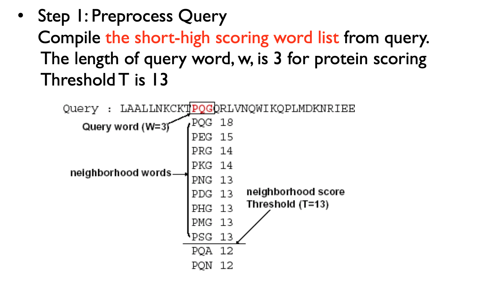
Basic Local Alignment Search Tool (Altschul et al., 1990 & 1997) is a sequence comparison algorithm optimized for speed used to search sequence databases for optimal local alignments to a query. The initial search is done for a word of length “W” that scores at least “T” when compared to the query using a substitution matrix. Word hits are then extended in either direction in an attempt to generate an alignment with a score exceeding the threshold of “S”. The “T” parameter dictates the speed and sensitivity of the search.
Rapidly compare a sequence Q to a database to find all sequences in the database with an score above some cutoff S.
- Which protein is most similar to a newly sequenced one?
- Where does this sequence of DNA originate?
- Speed achieved by using a procedure that typically finds most matches with scores > S.
- Tradeoff between sensitivity and specificity/speed
- Sensitivity – ability to find all related sequences
- Specificity – ability to reject unrelated sequences
Homologous sequence are likely to contain a short high scoring word pair, a seed.
– Unlike Baeza-Yates, BLAST doesn’t make explicit guarantees
BLAST then tries to extend high scoring word pairs to compute maximal high scoring segment pairs (HSPs).
– Heuristic algorithm but evaluates the result statistically.
E-value
E-value = the number of HSPs having score S (or higher) expected to occur by chance.
Smaller E-value, more significant in statistics Bigger E-value , by chance
E[# occurrences of a string of length m in reference of length L] ~ L/4m
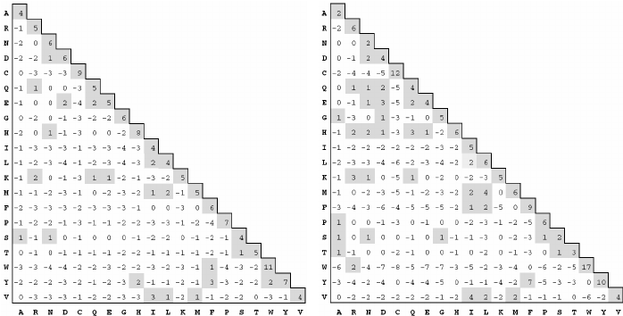
PAM and BLOSUM Matrices
Two different kinds of amino acid scoring matrices, PAM (Percent Accepted Mutation) and BLOSUM (BLOcks SUbstitution Matrix), are in wide use. The PAM matrices were created by Margaret Dayhoff and coworkers and are thus sometimes referred to as the Dayhoff matrices. These scoring matrices have a strong theoretical component and make a few evolutionary assumptions. The BLOSUM matrices, on the other hand, are more empirical and derive from a larger data set. Most researchers today prefer to use BLOSUM matrices because in silico experiments indicate that searches employing BLOSUM matrices have higher sensitivity.
There are several PAM matrices, each one with a numeric suffix. The PAM1 matrix was constructed with a set of proteins that were all 85 percent or more identical to one another. The other matrices in the PAM set were then constructed by multiplying the PAM1 matrix by itself: 100 times for the PAM100; 160 times for the PAM160; and so on, in an attempt to model the course of sequence evolution. Though highly theoretical (and somewhat suspect), it is certainly a reasonable approach. There was little protein sequence data in the 1970s when these matrices were created, so this approach was a good way to extrapolate to larger distances.
Protein databases contained many more sequences by the 1990s so a more empirical approach was possible. The BLOSUM matrices were constructed by extracting ungapped segments, or blocks, from a set of multiply aligned protein families, and then further clustering these blocks on the basis of their percent identity. The blocks used to derive the BLOSUM62 matrix, for example, all have at least 62 percent identity to some other member of the block.
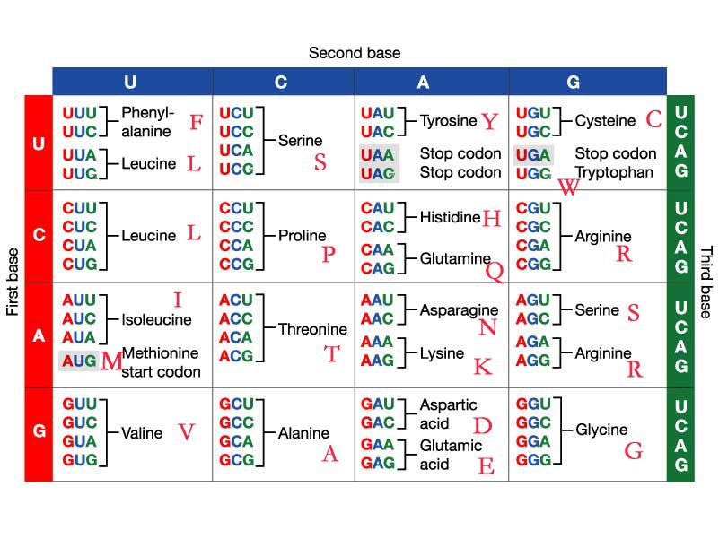
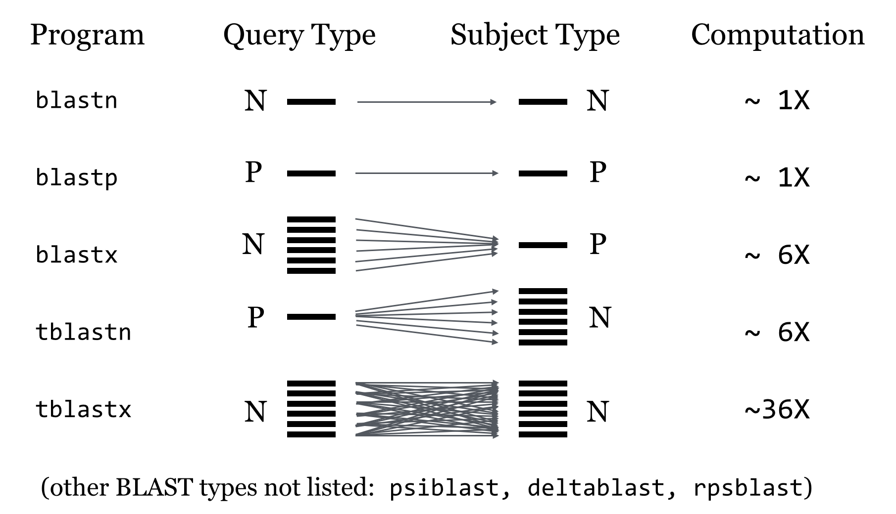
BLAST has a number of possible programs to run depending on whether you have nucleotide or protein sequences:
nucleotide query and nucleotide db - blastn nucleotide query and nucleotide db - tblastx (includes six frame translation of query and db sequences) nucleotide query and protein db - blastx (includes six frame translation of query sequences) protein query and nucleotide db - tblastn (includes six frame translation of db sequences) protein query and protein db - blastp
BLAST Process
NCBI BLAST
https://blast.ncbi.nlm.nih.gov/Blast.cgi
Uniprot
https://www.uniprot.org/
BLASTN example
Run blastn against the nt database.
ATGAAAGCGAAGGTTAGCCGTGGTGGCGGTTTTCGCGGTGCGCTGAACTA
CGTTTTTGACGTTGGCAAGGAAGCCACGCACACGAAAAACGCGGAGCGAG
TCGGCGGCAACATGGCCGGGAATGACCCCCGCGAACTGTCGCGGGAGTTC
TCAGCCGTGCGCCAGTTGCGCCCGGACATCGGCAAGCCCGTCTGGCATTG
CTCGCTGTCACTGCCTCCCGGCGAGCGCCTGAGCGCCGAGAAGTGGGAAG
CCGTCGCGGCTGACTTCATGCAGCGCATGGGCTTTGACCAGACCAATACG
CCGTGGGTGGCCGTGCGCCACCAGGACACGGACAAGGATCACATCCACAT
CGTGGCCAGCCGGGTAGGGCTGGACGGGAAAGTGTGGCTGGGCCAGTGGG
AAGCCCGCCGCGCCATCGAGGCGACCCAAGAGCTTGAGCATACCCACGGC
CTGACCCTGACGCCGGGGCTGGGCGATGCGCGGGCCGAGCGCCGGAAGCT
GACCGACAAGGAGATCAACATGGCCGTGAGAACGGGCGATGAACCGCCGC
GCCAGCGTCTGCAACGGCTGCTGGATGAGGCGGTGAAGGACAAGCCGACC
GCGCTAGAACTGGCCGAGCGGCTACAGGCCGCAGGCGTAGGCGTCCGGGC
AAACCTCGCCAGCACCGGGCGCATGAACGGCTTTTCCTTCGAGGTGGCCG
GAGTGCCGTTCAAAGGCAGCGACTTGGGCAAGGGCTACACATGGGCGGGG
CTACAGAAAGCAGGGGTGACTTATGACGAAGCTAGAGACCGTGCGGGCCT
TGAACGATTCAGGCCCACAGTTGCAGATCGTGGAGAGCGTCAGGACGTTG
CAGCAGTCCGTGAGCCTGATGCACGAGGACTTGAAGCGCCTACCGGGCGC
AGTCTCGACCGAGACGGCGCAGACCTTGGAACCGCTGGCCCGACTCCGGC
AGGACGTGACGCAGGTTCTGGAAGCCTACGACAAGGTGACGGCCATTCAG
CGCAAGACGCTGGACGAGCTGACGCAGCAGATGAGCGCGAGCGCGGCGCA
GGCCTTCGAGCAGAAGGCCGGGAAGCTGGACGCGACCATCTCCGACCTGT
CGCGCAGCCTGTCAGGGCTGAAAACGAGCCTCAGCAGCATGGAGCAGACC
GCGCAGCAGGTGGCGACCTTGCCGGGCAAGCTGGCGAGCGCACAGCAGGG
CATGACGAAAGCCGCCGACCAACTGACCGAGGCAGCGAACGAGACGCGCC
CGCGCCTTTGGCGGCAGGCGCTGGGGCTGATTCTGGCCGGGGCCGTGGGC
GCGATGCTGGTAGCGACTGGGCAAGTCGCTTTAAACAGGCTAGTGCCGCC
AAGCGACGTGCAGCAGACGGCAGACTGGGCCAACGCGATTTGGAACAAGG
CCACGCCCACGGAGCGCGAGTTGCTGAAACAGATCGCCAATCGGCCCGCG
AACTAGACCCGACCGCCTACCTTGAGGCCAGCGGCTACACCGTGAAGCGA
GAAGGGCGGCACCTGTCCGTCAGGGCGGGCGGTGATGAGGCGTACCGCGT
GACCCGGCAGCAGGACGGGCGCTGGCTCTGGTGCGACCGCTACGGCAACG
ACGGCGGGGACAATATCGACCTGGTGCGCGAGATCGAACCCGGCACCGGC
TACGCCGAGGCCGTCTATCGGCTTTCAGGTGCGCCGACAGTCCGGCAGCA
ACCGCGCCCGAGCGAGCCGAAGCGCCAACCGCCGCAGCTACCGGCGCAAG
GGCTGGCAGCCCGCGAGCATGGCCGCGACTACCTCAAGGGCCGGGGCATC
AGCCAGGACACCATCGAGCACGCCGAGAAGGCGGGCATGGTGCGCTATGC
AGACGGTGGAGTGCTGTTCGTCGGCTACGACCGTGCAGGCACCGCGCAGA
ACGCCACACGCCGCGCCATTGCCCCCGCTGACCCGGTGCAGAAGCGCGAC
CTACGCGGCAGCGACAAGAGCTATCCGCCGATCCTGCCGGGCGACCCGGC
AAAGGTCTGGATCGTGGAAGGTGGCCCGGATGCGCTGGCCCTGCACGACA
TCGCCAAGCGCAGCGGCCAGCAGCCGCCCACCGTCATCGTGTCAGGCGGG
GCGAACGTGCGCAGCTTCTTGGAGCGGGCCGACGTGCAAGCGATCCTGAA
GCGGGCCGAGCGCGTCACCGTGGCCGGGGAAAACGAGAAGAACCCCGAGG
CGCAGGCAAAGGCCGACGCCGGGCACCAGAAGCAGGCGCAGCGGGTGGCC
AAAATCACCGGGCGCGAGGTGCGCCAATGGACGCCGAAGCCCGAGCACGG
CAAGGACTTGGCCGACATGAACGCCCGGCAGGTGGCAGAGATCGAGCGCA
AGCGACAGGCCGAGATCGAGGCCGAAAGAGCACGAAACCGCGAGCTTTCA
CGCAAGAGCCGGAGGTATGATGGCCCCAGCTTCGGCAGATAA
BLASTP Query
Do a BLASTP on NCBI website with the following protein against nr, but limit the organism to cetartiodactyla using default parameters:
MASGPGGWLGPAFALRLLLAAVLQPVSAFRAEFSSESCRELGFSSNLLCSSCDLLGQFSL
LQLDPDCRGCCQEEAQFETKKYVRGSDPVLKLLDDNGNIAEELSILKWNTDSVEEFLSEK
LERI
Have a look at the multiple sequence alignment, can you explain the results?
Do a similar blastp vs UniProtKB (UniProt) without post filtering.
Running a standalone BLAST program
location
cd /data/gpfs/assoc/bch709-4/${USER}/BLAST
ENV
conda activate blast
Running a standalone BLAST program
Create the index for the target database using makeblastdb; Choose the task program: blastn, blastp, blastx, tblatx, psiblast or deltablast; Set the configuration for match, mismatch, gap-open penalty, gap-extension penalty or scoring matrix; Set the word size; Set the E-value threshold; Set the output format and the number of output results
Standalone BLAST
In addition to providing BLAST sequence alignment services on the web, NCBI also makes these sequence alignment utilities available for download through FTP. This allows BLAST searches to be performed on local platforms against databases downloaded from NCBI or created locally. These utilities run through DOS-like command windows and accept input through text-based command line switches. There is no graphic user interface
https://www.ncbi.nlm.nih.gov/books/NBK52640/
http://ftp.ncbi.nlm.nih.gov/blast/db/
NR vs NT
At NCBI they are two different things as well. ‘nr’ is a database of protein sequences and ‘nt’ is nucleotide. At one time ‘nr’ meant non-redundant but it stopped being non-redundant a while ago. nt is a nucleotide database, while nr is a protein database (in amino acids)
Standalone BLAST
- Download the database.
- Use makeblastdb to build the index.
- Change the scoring matrix, record the changes in the alignment results and interpret the results.
Download Database
wget ftp://ftp.ncbi.nih.gov/refseq/release/plant/plant.1.protein.faa.gz
How many sequences in plant.1.protein.faa.gz
Input file
/data/gpfs/assoc/bch709-4/Course_materials/BLAST/Athaliana_167_TAIR10.cds.fa.gz
Example Input sequence
seqkit stats /data/gpfs/assoc/bch709-4/Course_materials/BLAST/Athaliana_167_TAIR10.cds.fa.gz -T
file	format	type	num_seqs	sum_len	min_len	avg_len	max_len
/data/gpfs/assoc/bch709-4/Course_materials/BLAST/Athaliana_167_TAIR10.cds.fa.gz	FASTA	DNA	35386	43546761	22	1230.6	16182
Subsampling by SeqKit
FASTA and FASTQ are basic and ubiquitous formats for storing nucleotide and protein sequences. Common manipulations of FASTA/Q file include converting, searching, filtering, deduplication, splitting, shuffling, and sampling. Existing tools only implement some of these manipulations, and not particularly efficiently, and some are only available for certain operating systems. Furthermore, the complicated installation process of required packages and running environments can render these programs less user friendly.
This project describes a cross-platform ultrafast comprehensive toolkit for FASTA/Q processing. SeqKit provides executable binary files for all major operating systems, including Windows, Linux, and Mac OS X, and can be directly used without any dependencies or pre-configurations. SeqKit demonstrates competitive performance in execution time and memory usage compared to similar tools. The efficiency and usability of SeqKit enable researchers to rapidly accomplish common FASTA/Q file manipulations.
https://bioinf.shenwei.me/seqkit/
https://bioinf.shenwei.me/seqkit/tutorial/
Run BLAST
Make BLAST DB
makeblastdb -in your-nucleotide-db.fa -dbtype nucl
###for nucleotide sequence
makeblastdb -in your-protein-db.fas -dbtype prot
###for protein sequence
Run BLASTX
cd /data/gpfs/assoc/bch709-4/${USER}/BLAST
gunzip plant.1.protein.faa.gz
makeblastdb -in plant.1.protein.faa -dbtype prot
seqkit sample -n 100 /data/gpfs/assoc/bch709-4/Course_materials/BLAST/Athaliana_167_TAIR10.cds.fa.gz > ATH_100.fasta
blastx -query ATH_100.fasta  -db plant.1.protein.faa -outfmt 8
Tab output
qseqid 		Query sequence ID
sseqid		Subject (ie DB) sequence ID
pident		Percent Identity across the alignment
length 		Alignment length
mismatch 	# of mismatches
gapopen 	Number of gap openings
qstart 		Start of alignment in query
qend 		End of alignment in query
sstart 		Start of alignment in subject
send		End of alignment in subject
evalue 		E-value
bitscore	Bit score
Question
- find the option below within BLASTX
- Set output to file
- Set tabular output format
- Set maximum target sequence to one
- Set threads (CPU) to 32
- Set evalue threshold to 1e-30
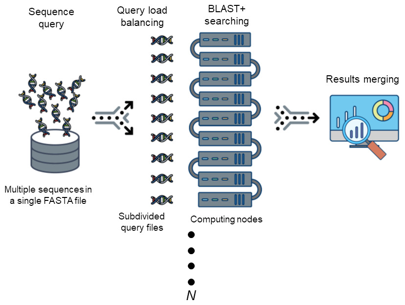
DCBLAST
The Basic Local Alignment Search Tool (BLAST) is by far best the most widely used tool in for sequence analysis for rapid sequence similarity searching among nucleic acid or amino acid sequences. Recently, cluster, HPC, grid, and cloud environmentshave been are increasing more widely used and more accessible as high-performance computing systems. Divide and Conquer BLAST (DCBLAST) has been designed to perform run on grid system with query splicing which can run National Center for Biotechnology Information (NCBI) BLASTBLAST search comparisons over withinthe cluster, grid, and cloud computing grid environment by using a query sequence distribution approach NCBI BLAST. This is a promising tool to accelerate BLAST job dramatically accelerates the execution of BLAST query searches using a simple, accessible, robust, and practical approach.
- DCBLAST can run BLAST job across HPC.
- DCBLAST suppport all NCBI-BLAST+ suite.
- DCBLAST generate exact same NCBI-BLAST+ result.
- DCBLAST can use all options in NCBI-BLAST+ suite.
Requirement
Following basic softwares are needed to run
- Perl (Any version 5+)
which perl
perl --version
- NCBI-BLAST+ (Any version) for easy approach, you can download binary version of blast from below link. ftp://ftp.ncbi.nlm.nih.gov/blast/executables/blast+/LATEST
For using recent version, please update BLAST path in config.ini
which blastn
- Sun Grid Engine (Any version)
which qsub - Slurm
which sbatch - Grid cloud or distributed computing system.
Prerequisites
The following Perl modules are required:
- Path::Tiny
- Data::Dumper
- Config::Tiny
Install prerequisites with the following command:
cpan `cat requirement`
or
cpanm `cat requirement`
or
cpanm Path::Tiny Data::Dumper Config::Tiny
We strongly recommend to use Perlbrew http://perlbrew.pl/ to avoid having to type sudo
We also recommend to use ‘cpanm’ https://github.com/miyagawa/cpanminus
Prerequisites by Conda
conda activate blast
conda install -c bioconda perl-path-tiny blast perl-data-dumper perl-config-tiny -y
Installation
The program is a single file Perl scripts. Copy it into executive directories.
We recommend to copy it on scratch disk.
cp /data/gpfs/assoc/bch709-4/Course_materials/BLAST/Athaliana_167_TAIR10.cds.fa.gz /data/gpfs/assoc/bch709-4/${USER}/BLAST

gunzip /data/gpfs/assoc/bch709-4/${USER}/BLAST/Athaliana_167_TAIR10.cds.fa.gz


cd /data/gpfs/assoc/bch709-4/${USER}/BLAST

mkdir /data/gpfs/assoc/bch709-4/${USER}/BLAST/

git clone git@github.com:wyim-pgl/DCBLAST.git

cd DCBLAST/DCBLAST-SLURM

pwd

chmod 775 dcblast.pl

perl dcblast.pl
Help
Usage : dcblast.pl --ini config.ini --input input-fasta --size size-of-group --output output-filename-prefix  --blast blast-program-name

  --ini <ini filename> ##config file ex)config.ini

  --input <input filename> ##query fasta file

  --size <output size> ## size of chunks usually all core x 2, if you have 160 core all nodes, you can use 320. please check it to your admin.

  --output <output filename> ##output folder name

  --blast <blast name> ##blastp, blastx, blastn and etcs.

  --dryrun Option will only split fasta file into chunks
Configuration
Please edit config.ini with nano before you run!!
[dcblast]
##Name of job (will use for SGE job submission name)
job_name_prefix=dcblast

[blast]
##BLAST options

##BLAST path (your blast+ path); $ which blastn; then remove "blastn"
path=~/miniconda3/envs/blast/bin/

##DB path (build your own BLAST DB)
##example
##makeblastdb -in example/test_db.fas -dbtype nucl (for nucleotide sequence)
##makeblastdb -in example/your-protein-db.fas -dbtype prot (for protein sequence)
db=/data/gpfs/assoc/bch709-4/${USER}/BLAST/plant.1.protein.faa

##Evalue cut-off (See BLAST manual)
evalue=1e-05

##number of threads in each job. If your CPU is AMD it needs to be set 1.
num_threads=2

##Max target sequence output (See BLAST manual)
max_target_seqs=10

##Output format (See BLAST manual)
outfmt=6

##any other option can be add it this area
#matrix=BLOSUM62
#gapopen=11
#gapextend=1

[oldsge]
##Grid job submission commands
##please check your job submission scripts
##Especially Queue name (q) and Threads option (pe) will be different depends on your system

pe=SharedMem 1
M=your@email
q=common.q
j=yes
o=log
cwd=

[slurm]
time=04:00:00
cpus-per-task=1
mem-per-cpu=800M
ntasks=1
output=log
error=error
partition=cpu-core-0
account=cpu-s5-bch709-4
mail-type=all
mail-user=${USER}@unr.edu
If you need any other options for your enviroment please contant us or admin
PBS & LSF need simple code hack. If you need it please request through issue.
Run DCBLAST
Run (–dryrun option will only split fasta file into chunks)
perl dcblast.pl --ini config.ini --input /data/gpfs/assoc/bch709-4/${USER}/BLAST/Athaliana_167_TAIR10.cds.fa --output test --size 100 --blast blastx
squeue
It usually finish within up to 20min depends on HPC status and CPU speed.
Citation
Won C. Yim and John C. Cushman (2017) Divide and Conquer BLAST: using grid engines to accelerate BLAST and other sequence analysis tools. PeerJ 10.7717/peerj.3486 https://peerj.com/articles/3486/