15_RNA-Seq tutorial III – BCH709 Introduction to Bioinformatics

WORKTING PATH

mkdir /data/gpfs/assoc/bch709-1/<YOURID>/RNA-Seq_example/
cd /data/gpfs/assoc/bch709-1/<YOURID>/RNA-Seq_example/

Conda environment

CONDA_INSTRUMENTATION_ENABLED=1 conda create -n BCH709 python=3.7

conda activate BCH709

CONDA_INSTRUMENTATION_ENABLED=1 conda install -y -c bioconda -c conda-forge  sra-tools minimap2 trinity star multiqc=1.9 samtools=1.9 trim-galore gffread seqkit kraken2

CONDA_INSTRUMENTATION_ENABLED=1 conda install -y -c bioconda -c conda-forge -c r openssl=1.0 r-base icu=58.2 bioconductor-ctc  bioconductor-deseq2=1.20.0 bioconductor-biobase=2.40.0  bioconductor-qvalue=2.16.0 r-ape  r-gplots r-fastcluster=1.1.25 libiconv

GTF format

The Gene Transfer Format (GTF) is a widely used format for storing gene annotations. You can obtain GTF files easily from the UCSC table browser and Ensembl

Fields must be tab-separated. Also, all but the final field in each feature line must contain a value; “empty” columns should be denoted with a ‘.’

seqname - name of the chromosome or scaffold; chromosome names can be given with or without the ‘chr’ prefix. Important note: the seqname must be one used within Ensembl, i.e. a standard chromosome name or an Ensembl identifier such as a scaffold ID, without any additional content such as species or assembly. See the example GFF output below.
source - name of the program that generated this feature, or the data source (database or project name)
feature - feature type name, e.g. Gene, Variation, Similarity
start - Start position of the feature, with sequence numbering starting at 1.
end - End position of the feature, with sequence numbering starting at 1.
score - A floating point value.
strand - defined as + (forward) or - (reverse).
frame - One of ‘0’, ‘1’ or ‘2’. ‘0’ indicates that the first base of the feature is the first base of a codon, ‘1’ that the second base is the first base of a codon, and so on..
attribute - A semicolon-separated list of tag-value pairs, providing additional information about each feature.

Arabidopsis

Environment

conda activate BCH709

CONDA_INSTRUMENTATION_ENABLED=1 conda install -c bioconda intervene pybedtools pandas seaborn bedtools subread -y

CONDA_INSTRUMENTATION_ENABLED=1 conda install -y -c bioconda -c conda-forge  sra-tools minimap2 trinity star multiqc=1.9 samtools=1.9 trim-galore gffread seqkit kraken2

CONDA_INSTRUMENTATION_ENABLED=1 conda install -c r r-UpSetR r-corrplot r-Cairo r-ape   -y

conda update --all

CONDA_INSTRUMENTATION_ENABLED=1 conda install -y -c bioconda r-gplots r-fastcluster=1.1.25  bioconductor-ctc  bioconductor-deseq2 bioconductor-biobase=2.40.0  bioconductor-qvalue  bioconductor-limma bioconductor-edger  bioconductor-genomeinfodb bioconductor-deseq2 bioconductor-genomeinfodbdata r-rcurl

Working PATH

conda activate BCH709
cd /data/gpfs/assoc/bch709-1/<YOURID>/RNA-Seq_example/ATH

Reads count

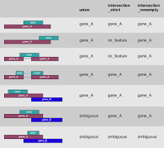
In the case of RNA-Seq, the features are typically genes, where each gene is considered here as the union of all its exons. Counting RNA-seq reads is complex because of the need to accommodate exon splicing. The common approach is to summarize counts at the gene level, by counting all reads that overlap any exon for each gene. In this method, gene annotation file from RefSeq or Ensembl is often used for this purpose. So far there are two major feature counting tools: featureCounts (Liao et al.) and htseq-count (Anders et al.)

featurecount

mkdir DEG
cd bam

ls -1 *.bam

ls -1 *.bam |  tr '\n' ' '

nano readscount.sh

#!/bin/bash
#SBATCH --job-name=featureCounts
#SBATCH --cpus-per-task=16
#SBATCH --time=15:00
#SBATCH --mem=20g
#SBATCH --mail-type=all
#SBATCH --mail-user=<EMAIL>@unr.edu
#SBATCH -o featureCounts.out # STDOUT
#SBATCH -e featureCounts.err # STDERR
#SBATCH -p cpu-s2-core-0 
#SBATCH -A cpu-s2-bch709-1
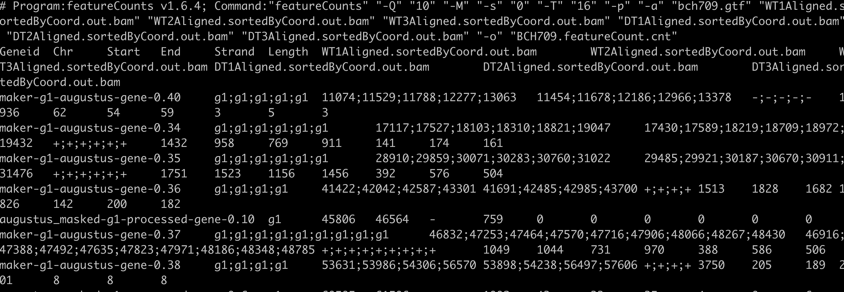
featureCounts -Q 10 -M -s 0 -T 16 -p -a /data/gpfs/assoc/bch709-1/<YOURID>/RNA-Seq_example/ATH/reference/TAIR10_GFF3_genes.gtf SRR1761506.bamAligned.sortedByCoord.out.bam SRR1761507.bamAligned.sortedByCoord.out.bam SRR1761508.bamAligned.sortedByCoord.out.bam SRR1761509.bamAligned.sortedByCoord.out.bam SRR1761510.bamAligned.sortedByCoord.out.bam SRR1761511.bamAligned.sortedByCoord.out.bam -o ATH.featureCount.cnt

featureCounts -g transcript_id -t transcript -f  -Q 10 -M -s 0 -T 16 -p -a /data/gpfs/assoc/bch709-1/<YOURID>/RNA-Seq_example/ATH/reference/TAIR10_GFF3_genes.gtf SRR1761506.bamAligned.sortedByCoord.out.bam SRR1761507.bamAligned.sortedByCoord.out.bam SRR1761508.bamAligned.sortedByCoord.out.bam SRR1761509.bamAligned.sortedByCoord.out.bam SRR1761510.bamAligned.sortedByCoord.out.bam SRR1761511.bamAligned.sortedByCoord.out.bam -o ATH.featureCount_isoform.cnt

featurecount2

sed -i 's/<YOURID>/\t/g' readscount.sh

head ATH.featureCount.cnt

cut -f1,7-  ATH.featureCount.cnt |  egrep -v "#" | sed 's/\Aligned\.sortedByCoord\.out\.bam//g; s/\.bam//g' >> ATH.featureCount_count_only.cnt

Go to DEG

cd ../DEG
cp ../bam/ATH.featureCount* .
ls

pwd

/data/gpfs/assoc/bch709-1/<YOURID>/RNA-Seq_example/ATH/DEG

Data list

Sample information	Run
WT_rep1	SRR1761506
WT_rep2	SRR1761507
WT_rep3	SRR1761508
ABA_rep1	SRR1761509
ABA_rep2	SRR1761510
ABA_rep3	SRR1761511

sample files

nano samples.txt

WT<TAB>SRR1761506
WT<TAB>SRR1761507
WT<TAB>SRR1761508
ABA<TAB>SRR1761509
ABA<TAB>SRR1761510
ABA<TAB>SRR1761511

sed -i 's/<TAB>/\t/g' samples.txt

PtR (Quality Check Your Samples and Biological Replicates)

Once you’ve performed transcript quantification for each of your biological replicates, it’s good to examine the data to ensure that your biological replicates are well correlated, and also to investigate relationships among your samples. If there are any obvious discrepancies among your sample and replicate relationships such as due to accidental mis-labeling of sample replicates, or strong outliers or batch effects, you’ll want to identify them before proceeding to subsequent data analyses (such as differential expression).

PtR  --matrix ATH.featureCount_count_only.cnt  --samples samples.txt --CPM  --log2 --min_rowSums 10   --sample_cor_matrix --compare_replicates

WT.rep_compare.pdf
ABA.rep_compare.pdf

DEG calculation

install.packages("blob")

if (!requireNamespace("BiocManager", quietly = TRUE))
    install.packages("BiocManager")

BiocManager::install(c("GenomeInfoDb","DESeq2"))

quit()

run_DE_analysis.pl --matrix ATH.featureCount_count_only.cnt --method DESeq2 --samples_file samples.txt --output rnaseq

DEG output

ls rnaseq

ATH.featureCount_count_only.cnt.ABA_vs_WT.DESeq2.count_matrix
ATH.featureCount_count_only.cnt.ABA_vs_WT.DESeq2.DE_results
ATH.featureCount_count_only.cnt.ABA_vs_WT.DESeq2.DE_results.MA_n_Volcano.pdf
ATH.featureCount_count_only.cnt.ABA_vs_WT.DESeq2.Rscript

TPM and FPKM calculation

cut -f1,6-  ATH.featureCount.cnt |  egrep -v "#" | sed 's/\Aligned\.sortedByCoord\.out\.bam//g; s/\.bam//g' > ATH.featureCount_count_length.cnt

python /data/gpfs/assoc/bch709-1/Course_material/script/tpm_raw_exp_calculator.py -count ATH.featureCount_count_length.cnt

TPM and FPKM calculation output

ATH.featureCount_count_length.cnt.fpkm.xls
ATH.featureCount_count_length.cnt.fpkm.tab
ATH.featureCount_count_length.cnt.tpm.xls
ATH.featureCount_count_length.cnt.tpm.tab

DEG subset

cd rnaseq
analyze_diff_expr.pl --samples ../samples.txt  --matrix ../ATH.featureCount_count_length.cnt.tpm.tab -P 0.01 -C 2 --output ATH
analyze_diff_expr.pl --samples ../samples.txt  --matrix ../ATH.featureCount_count_length.cnt.tpm.tab -P 0.01 -C 1 --output ATH

DEG output

ATH.matrix.log2.centered.sample_cor_matrix.pdf
ATH.matrix.log2.centered.genes_vs_samples_heatmap.pdf

ATH.featureCount_count_only.cnt.ABA_vs_WT.DESeq2.DE_results.P0.01_C2.ABA-UP.subset
ATH.featureCount_count_only.cnt.ABA_vs_WT.DESeq2.DE_results.P0.01_C2.WT-UP.subset
ATH.featureCount_count_only.cnt.ABA_vs_WT.DESeq2.DE_results.P0.01_C2.DE.subset

ATH.featureCount_count_only.cnt.ABA_vs_WT.DESeq2.DE_results.P0.01_C1.ABA-UP.subset
ATH.featureCount_count_only.cnt.ABA_vs_WT.DESeq2.DE_results.P0.01_C1.WT-UP.subset
ATH.featureCount_count_only.cnt.ABA_vs_WT.DESeq2.DE_results.P0.01_C1.DE.subset

Draw Venn Diagram

Venn Diagram

conda activate venn

Venn Diagram environment creation

conda create -n venn python=3.5
conda activate venn
conda install -c bioconda bedtools intervene r-UpSetR=1.4.0 r-corrplot r-Cairo

# /data/gpfs/assoc/bch709-1/<YOURID>/RNA-Seq_example/ATH/DEG/rnaseq
mkdir venn
cd venn
#/data/gpfs/assoc/bch709-1/<YOURID>/RNA-Seq_example/ATH/DEG/rnaseq/venn

cut -f 1 ../ATH.featureCount_count_only.cnt.ABA_vs_WT.DESeq2.DE_results.P0.01_C2.ABA-UP.subset |  grep -v sample > DESeq.UP_4fold.subset
cut -f 1 ../ATH.featureCount_count_only.cnt.ABA_vs_WT.DESeq2.DE_results.P0.01_C2.WT-UP.subset  |  grep -v sample > DESeq.DOWN_4fold.subset 

cut -f 1 ../ATH.featureCount_count_only.cnt.ABA_vs_WT.DESeq2.DE_results.P0.01_C1.ABA-UP.subset |  grep -v sample > DESeq.UP_2fold.subset
cut -f 1 ../ATH.featureCount_count_only.cnt.ABA_vs_WT.DESeq2.DE_results.P0.01_C1.WT-UP.subset  |  grep -v sample > DESeq.DOWN_2fold.subset

 wc -l *

DESeq.DOWN_2fold.subset
DESeq.DOWN_4fold.subset
DESeq.UP_2fold.subset
DESeq.UP_4fold.subset
total

intervene venn --type list --save-overlaps -i <INPUT> 
intervene upset --type list --save-overlaps -i <INPUT> 

cd Intervene_results

Intervene_upset_combinations.txt
Intervene_upset.pdf
Intervene_upset.R
Intervene_venn.pdf
sets

cd sets

0010_DESeq.UP_2fold.txt
0011_DESeq.UP_2fold_DESeq.UP_4fold.txt
1000_DESeq.DOWN_2fold.txt
1100_DESeq.DOWN_2fold_DESeq.DOWN_4fold.txt

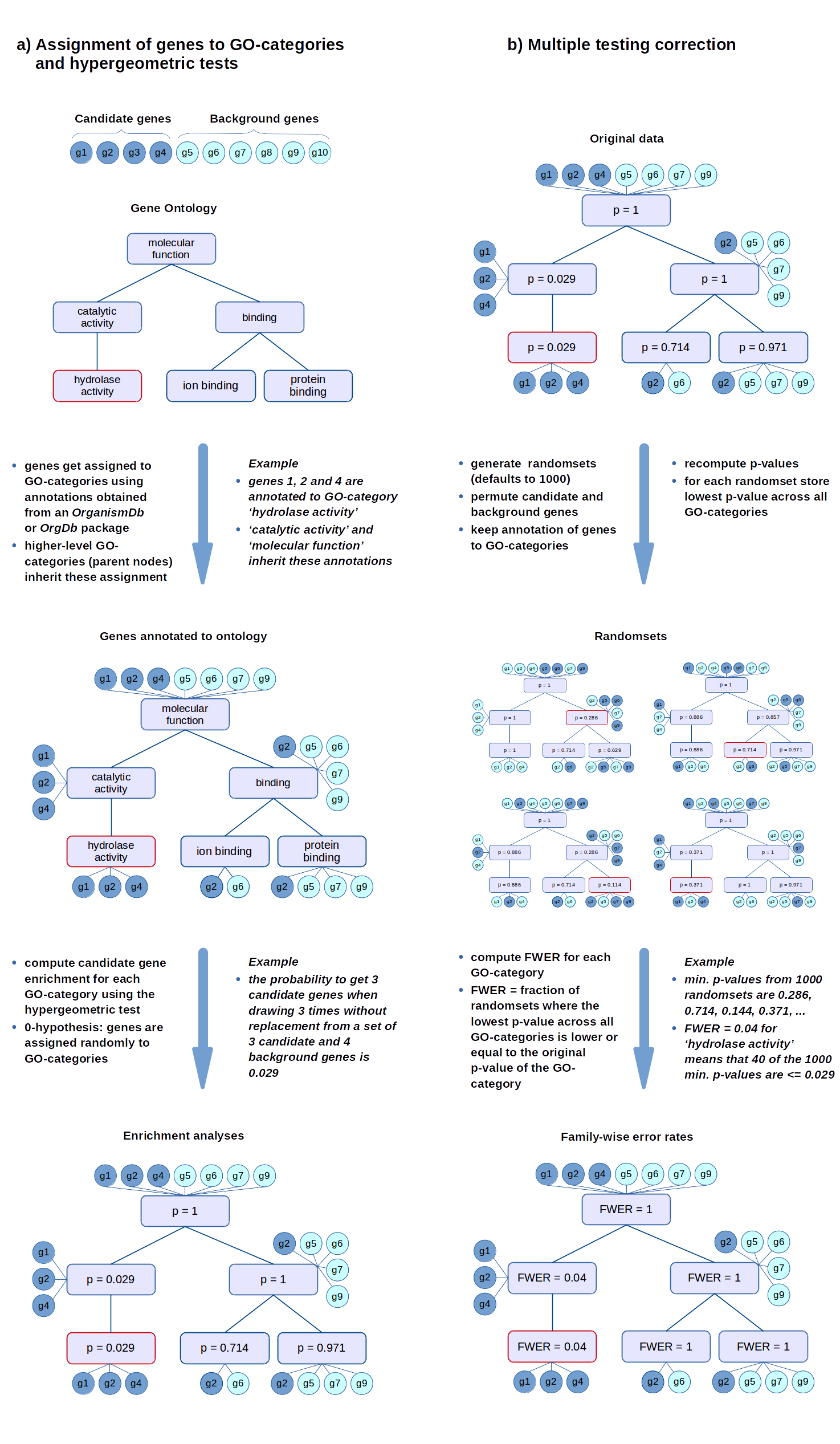
Gene Ontology

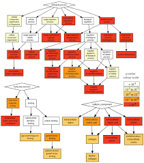
Gene Ontology project is a major bioinformatics initiative Gene ontology is an annotation system The project provides the controlled and consistent vocabulary of terms and gene product annotations, i.e. terms occur only once, and there is a dictionary of allowed words GO describes how gene products behave in a cellular context A consistent description of gene products attributes in terms of their associated biological processes, cellular components and molecular functions in a species-independent manner Each GO term consists of a unique alphanumerical identifier, a common name, synonyms (if applicable), and a definition Each term is assigned to one of the three ontologies Terms have a textual definition When a term has multiple meanings depending on species, the GO uses a “sensu” tag to differentiate among them (trichome differentiation (sensu Magnoliophyta)

kegg

hypergeometric test

The hypergeometric distribution is the lesser-known cousin of the binomial distribution, which describes the probability of k successes in n draws with replacement. The hypergeometric distribution describes probabilities of drawing marbles from the jar without putting them back in the jar after each draw. The hypergeometric probability mass function is given by (using the original variable convention)

hyper_geo combination FWER

FWER

The FWER for the other tests is computed in the same way: the gene-associated variables (scores or counts) are permuted while the annotations of genes to GO-categories stay fixed. Then the statistical tests are evaluated again for every GO-category.

Hypergeometric Test Example 1

Suppose we randomly select 2 cards without replacement from an ordinary deck of playing cards. What is the probability of getting exactly 2 cards you want (i.e., Ace or 10)?

Solution: This is a hypergeometric experiment in which we know the following:

N = 52; since there are 52 cards in a deck. k = 16; since there are 16 Ace or 10 cards in a deck. n = 2; since we randomly select cards from the deck. x = 2; since 2 of the cards we select are red. We plug these values into the hypergeometric formula as follows:

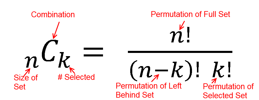
h(x; N, n, k) = [ kCx ] [ N-kCn-x ] / [ NCn ]

h(2; 52, 2, 16) = [ 16C2 ] [ 48C1 ] / [ 52C2 ]

h(2; 52, 2, 16) = [ 325 ] [ 1 ] / [ 1,326 ]

h(2; 52, 2, 16) = 0.0904977

Thus, the probability of randomly selecting 2 Ace or 10 cards is 9%

category	probability
probability mass f	0.09049773755656108597285
lower cumulative P	1
upper cumulative Q	0.09049773755656108597285
Expectation	0.6153846153846153846154

Hypergeometric Test Example 2

Suppose we have 30 DEGs in human genome (200). What is the probability of getting 10 oncogene?

An oncogene is a gene that has the potential to cause cancer.

Solution: This is a hypergeometric experiment in which we know the following:

N = 200; since there are 200 genes in human genome k = 10; since there are 10 oncogenes in human n = 30; since 30 DEGs x = 5; since 5 of the oncogenes in DEGs.

We plug these values into the hypergeometric formula as follows:

h(x; N, n, k) = [ kCx ] [ N-kCn-x ] / [ NCn ]

h(5; 200, 30, 10) = [ 10C5 ] [ 190C25 ] / [ 200C30 ]

h(5; 200, 30, 10) = [ 252 ] [ 11506192278177947613740456466942 ] / [ 409681705022127773530866523638950880 ]

h(5; 200, 30, 10) = 0.007078

Thus, the probability of oncogene 0.7%.

hypergeometry.png

hypergeometric distribution value

category	probability
probability mass f	0.0070775932109153651831923063371216961166297
lower cumulative P	0.99903494867072865323201131115533112651846
upper cumulative Q	0.0080426445401867119511809951817905695981658
Expectation	1.5

False Discovery Rate (FDR) q-value

The false discovery rate (FDR) is a method of conceptualizing the rate of type I errors in null hypothesis testing when conducting multiple comparisons. FDR-controlling procedures are designed to control the expected proportion of “discoveries” (rejected null hypotheses) that are false (incorrect rejections).

Benjamini–Yekutieli
Benjamini–Hochberg
Bonferroni-Selected–Bonferroni
Bonferroni and Sidak

REViGO

http://revigo.irb.hr/revigo.jsp

cleverGO

http://www.tartaglialab.com/GO_analyser/tutorial

MetaScape

http://metascape.org/gp/index.html

DAVID

https://david.ncifcrf.gov/

Araport

http://araport.org

Drosophila

cd /data/gpfs/assoc/bch709-1/<YOURID>/RNA-Seq_example/Drosophila/

Environment

conda activate BCH709

CONDA_INSTRUMENTATION_ENABLED=1 conda install -c bioconda intervene pybedtools pandas seaborn bedtools subread -y

CONDA_INSTRUMENTATION_ENABLED=1 conda install -y -c bioconda -c conda-forge  sra-tools minimap2 trinity star multiqc=1.9 samtools=1.9 trim-galore gffread seqkit kraken2

CONDA_INSTRUMENTATION_ENABLED=1 conda install -c r r-UpSetR r-corrplot r-Cairo r-ape   -y

conda update --all

CONDA_INSTRUMENTATION_ENABLED=1 conda install -y -c bioconda r-gplots r-fastcluster=1.1.25  bioconductor-ctc  bioconductor-deseq2 bioconductor-biobase=2.40.0  bioconductor-qvalue  bioconductor-limma bioconductor-edger  bioconductor-genomeinfodb bioconductor-deseq2 bioconductor-genomeinfodbdata r-rcurl

Working PATH

conda activate BCH709
cd /data/gpfs/assoc/bch709-1/<YOURID>/RNA-Seq_example/Drosophila/

mkdir DEG
cd bam

ls -1 *.bam

ls -1 *.bam |  tr '\n' ' '

nano readscount.sh

#!/bin/bash
#SBATCH --job-name=featureCounts
#SBATCH --cpus-per-task=16
#SBATCH --time=15:00
#SBATCH --mem=20g
#SBATCH --mail-type=all
#SBATCH --mail-user=<EMAIL>@unr.edu
#SBATCH -o featureCounts.out # STDOUT
#SBATCH -e featureCounts.err # STDERR
#SBATCH -p cpu-s2-core-0 
#SBATCH -A cpu-s2-bch709-1
featureCounts -g transcript_symbol -t mRNA -f  -M -s 0 -T 16 -a /data/gpfs/assoc/bch709-1/<YOURID>/RNA-Seq_example/Drosophila/reference/dmel-all-r6.36.gtf SRR11968954.bamAligned.sortedByCoord.out.bam SRR11968962.bamAligned.sortedByCoord.out.bam SRR11968963.bamAligned.sortedByCoord.out.bam SRR11968964.bamAligned.sortedByCoord.out.bam SRR11968965.bamAligned.sortedByCoord.out.bam SRR11968966.bamAligned.sortedByCoord.out.bam -o dmel.featureCount.cnt

sed -i 's/<YOURID>/\t/g' readscount.sh

head dmel.featureCount.cnt

cut -f1,7-  dmel.featureCount.cnt |  egrep -v "#" | sed 's/\Aligned\.sortedByCoord\.out\.bam//g; s/\.bam//g' > dmel.featureCount_count_only.cnt

Go to DEG

cd ../DEG
cp ../bam/dmel.featureCount* .
ls

pwd

/data/gpfs/assoc/bch709-1/<YOURID>/RNA-Seq_example/Drosophila/DEG

Data list

Sample information	Run
22w1118-l3	SRR11968964
23w1118-l3	SRR11968963
24w1118-l3	SRR11968962
10w1118-sa	SRR11968954
11w1118-sa	SRR11968966
12w1118-sa	SRR11968965

sample files

nano samples.txt

l3<TAB>SRR11968964
l3<TAB>SRR11968963
l3<TAB>SRR11968962
sa<TAB>SRR11968954
sa<TAB>SRR11968966
sa<TAB>SRR11968965

sed -i 's/<TAB>/\t/g' samples.txt

PtR (Quality Check Your Samples and Biological Replicates)

PtR  --matrix dmel.featureCount_count_only.cnt  --samples samples.txt --CPM  --log2 --min_rowSums 10   --sample_cor_matrix --compare_replicates

Will give you error

DEG calculation

run_DE_analysis.pl --matrix dmel.featureCount_count_only.cnt --method DESeq2 --samples_file samples.txt --output rnaseq

If you have an error, Please do this

conda install -c conda-forge xorg-libxt

install.packages(c("blob","stringi"))
source("https://bioconductor.org/biocLite.R")

BiocInstaller::biocLite(c("GenomeInfoDbData","DESeq2"))
quit()

DEG output

ls rnaseq

dmel.featureCount_count_only.cnt.l3_vs_sa.DESeq2.count_matrix
dmel.featureCount_count_only.cnt.l3_vs_sa.DESeq2.DE_results
dmel.featureCount_count_only.cnt.l3_vs_sa.DESeq2.DE_results.MA_n_Volcano.pdf
dmel.featureCount_count_only.cnt.l3_vs_sa.DESeq2.Rscript

TPM and FPKM calculation

cut -f1,6-  dmel.featureCount.cnt |  egrep -v "#" | sed 's/\Aligned\.sortedByCoord\.out\.bam//g; s/\.bam//g' > dmel.featureCount_count_length.cnt

python /data/gpfs/assoc/bch709-1/Course_material/script/tpm_raw_exp_calculator.py -count dmel.featureCount_count_length.cnt

If you have an error, Please do this

conda install -c bioconda -c conda-forge pandas

TPM and FPKM calculation output

dmel.featureCount_count_length.cnt
dmel.featureCount_count_length.cnt.fpkm.tab
dmel.featureCount_count_length.cnt.fpkm.xls
dmel.featureCount_count_length.cnt.tpm.tab
dmel.featureCount_count_length.cnt.tpm.xls

DEG subset

cd rnaseq
analyze_diff_expr.pl --samples ../samples.txt  --matrix ../dmel.featureCount_count_length.cnt.tpm.tab -P 0.01 -C 2 --output dmel
analyze_diff_expr.pl --samples ../samples.txt  --matrix ../dmel.featureCount_count_length.cnt.tpm.tab -P 0.01 -C 1 --output dmel

DEG output

dmel.featureCount_count_only.cnt.l3_vs_sa.DESeq2.DE_results.MA_n_Volcano.pdf
dmel.featureCount_count_only.cnt.l3_vs_sa.DESeq2.DE_results.P0.01_C1.DE.subset
dmel.featureCount_count_only.cnt.l3_vs_sa.DESeq2.DE_results.P0.01_C1.l3-UP.subset
dmel.featureCount_count_only.cnt.l3_vs_sa.DESeq2.DE_results.P0.01_C1.sa-UP.subset
dmel.featureCount_count_only.cnt.l3_vs_sa.DESeq2.DE_results.P0.01_C2.DE.subset
dmel.featureCount_count_only.cnt.l3_vs_sa.DESeq2.DE_results.P0.01_C2.l3-UP.subset
dmel.featureCount_count_only.cnt.l3_vs_sa.DESeq2.DE_results.P0.01_C2.sa-UP.subset
dmel.featureCount_count_only.cnt.l3_vs_sa.DESeq2.DE_results.samples
dmel.featureCount_count_only.cnt.l3_vs_sa.DESeq2.Rscript

Draw Venn Diagram

Venn Diagram

conda activate venn

# /data/gpfs/assoc/bch709-1/<YOURID>/RNA-Seq_example/Drosophila/DEG/rnaseq
mkdir venn
cd venn
#/data/gpfs/assoc/bch709-1/<YOURID>/RNA-Seq_example/Drosophila/DEG/rnaseq/venn

cut -f 1 ../dmel.featureCount_count_only.cnt.l3_vs_sa.DESeq2.DE_results.P0.01_C2.l3-UP.subset |  grep -v sample > DESeq.UP_4fold.subset
cut -f 1 ../dmel.featureCount_count_only.cnt.l3_vs_sa.DESeq2.DE_results.P0.01_C2.sa-UP.subset  |  grep -v sample > DESeq.DOWN_4fold.subset 

cut -f 1 ../dmel.featureCount_count_only.cnt.l3_vs_sa.DESeq2.DE_results.P0.01_C1.l3-UP.subset |  grep -v sample > DESeq.UP_2fold.subset
cut -f 1 ../dmel.featureCount_count_only.cnt.l3_vs_sa.DESeq2.DE_results.P0.01_C1.sa-UP.subset  |  grep -v sample > DESeq.DOWN_2fold.subset

 wc -l *

DESeq.DOWN_2fold.subset
DESeq.DOWN_4fold.subset
DESeq.UP_2fold.subset
DESeq.UP_4fold.subset
total

intervene venn --type list --save-overlaps -i <INPUT> 
intervene upset --type list --save-overlaps -i <INPUT> 

cd Intervene_results

Intervene_upset_combinations.txt
Intervene_upset.pdf
Intervene_upset.R
Intervene_venn.pdf
sets

cd sets

0010_DESeq.UP_2fold.txt
0011_DESeq.UP_2fold_DESeq.UP_4fold.txt
1000_DESeq.DOWN_2fold.txt
1100_DESeq.DOWN_2fold_DESeq.DOWN_4fold.txt

Metascape

https://metascape.org/gp/index.html

Sequence sampling

cd /data/gpfs/assoc/bch709-1/<YOURID>/RNA-Seq_example/Drosophila/

seqkit sample  --number 5 /data/gpfs/assoc/bch709-1/<YOURID>/RNA-Seq_example/Drosophila/reference/dmel-all-CDS-r6.36.fasta -o random.fasta

seqkit translate random.fasta -o random.aa

BLAST (Basic Local Alignment Search Tool)

BLAST is a popular program for searching biosequences against databases. BLAST was developed and is maintained by a group at the National Center for Biotechnology Information (NCBI). Salient characteristics of BLAST are:

Local alignments

BLAST tries to find patches of regional similarity, rather than trying to find the best alignment between your entire query and an entire database sequence.

Ungapped alignments

Alignments generated with BLAST do not contain gaps. BLAST’s speed and statistical model depend on this, but in theory it reduces sensitivity. However, BLAST will report multiple local alignments between your query and a database sequence.

Explicit statistical theory

BLAST is based on an explicit statistical theory developed by Samuel Karlin and Steven Altschul (PNAS 87:2284-2268. 1990) The original theory was later extended to cover multiple weak matches between query and database entry PNAS 90:5873. 1993).

CAUTION: the repetitive nature of many biological sequences (particularly naive translations of DNA/RNA) violates assumptions made in the Karlin & Altschul theory. While the P values provided by BLAST are a good rule-of-thumb for initial identification of promising matches, care should be taken to ensure that matches are not due simply to biased amino acid composition.

CAUTION: The databases are contaminated with numerous artifacts. The intelligent use of filters can reduce problems from these sources. Remember that the statistical theory only covers the likelihood of finding a match by chance under particular assumptions; it does not guarantee biological importance.

Heuristic

BLAST is not guaranteed to find the best alignment between your query and the database; it may miss matches. This is because it uses a strategy which is expected to find most matches, but sacrifices complete sensitivity in order to gain speed. However, in practice few biologically significant matches are missed by BLAST which can be found with other sequence search programs. BLAST searches the database in two phases. First it looks for short subsequences which are likely to produce significant matches, and then it tries to extend these subsequences. A substitution matrix is used during all phases of protein searches (BLASTP, BLASTX, TBLASTN) Both phases of the alignment process (scanning & extension) use a substitution matrix to score matches. This is in contrast to FASTA, which uses a substitution matrix only for the extension phase. Substitution matrices greatly improve sensitivity.

Popular BLAST software

BLASTP

search a Protein Sequence against a Protein Database.

BLASTN

search a Nucleotide Sequence against a Nucleotide Database.

TBLASTN

search a Protein Sequence against a Nucleotide Database, by translating each database Nucleotide sequence in all 6 reading frames.

BLASTX

search a Nucleotide Sequence against a Protein Database, by first translating the query Nucleotide sequence in all 6 reading frames.

BLAST site

https://blast.ncbi.nlm.nih.gov/Blast.cgi https://www.uniprot.org/

Assignment

Please upload below files by 12/06/20 to Webcampus

Arabidopsis RNA-Seq analysis

WT.rep_compare.pdf
ABA.rep_compare.pdf
ATH.featureCount_count_only.cnt.ABA_vs_WT.DESeq2.DE_results.MA_n_Volcano.pdf
ATH.matrix.log2.centered.sample_cor_matrix.pdf
ATH.matrix.log2.centered.genes_vs_samples_heatmap.pdf
Intervene_upset.pdf
Intervene_venn.pdf

Drosophila RNA-Seq analysis
dmel.featureCount_count_only.cnt.l3_vs_sa.DESeq2.DE_results.MA_n_Volcano.pdf
Intervene_upset.pdf
Intervene_venn.pdf

BCH709 Introduction to Bioinformatics: 15_RNA-Seq tutorial III

WORKTING PATH

Conda environment

GTF format

Arabidopsis

Environment

Working PATH

Reads count

Go to DEG

Data list

sample files

PtR (Quality Check Your Samples and Biological Replicates)

DEG calculation

DEG output

TPM and FPKM calculation

TPM and FPKM calculation output

DEG subset

DEG output

Draw Venn Diagram

Venn Diagram

Venn Diagram environment creation

Gene Ontology

hypergeometric test

FWER

Hypergeometric Test Example 1

Hypergeometric Test Example 2

hypergeometric distribution value

False Discovery Rate (FDR) q-value

REViGO

cleverGO

MetaScape

DAVID

Araport

Drosophila

Environment

Working PATH

Go to DEG

Data list

sample files

PtR (Quality Check Your Samples and Biological Replicates)

DEG calculation

If you have an error, Please do this

DEG output

TPM and FPKM calculation

If you have an error, Please do this

TPM and FPKM calculation output

DEG subset

DEG output

Draw Venn Diagram

Venn Diagram

Metascape

Sequence sampling

BLAST (Basic Local Alignment Search Tool)

Local alignments

Ungapped alignments

Explicit statistical theory

Heuristic

Popular BLAST software

BLASTP

BLASTN

TBLASTN

BLASTX

BLAST site

Assignment