Environment creation
conda create -n BCH709_RNASeq -c bioconda -c conda-forge -c anaconda python=3.7 mamba

conda activate BCH709_RNASeq

mamba install -c bioconda -c conda-forge -c anaconda trim-galore=0.6.7 sra-tools=2.11.0 STAR htseq=1.99.2 subread=2.0.1 multiqc=1.11 snakemake=7.5.0 parallel-fastq-dump=0.6.7 bioconductor-tximport samtools=1.14 r-ggplot2 trinity=2.13.2 hisat2 bioconductor-qvalue sambamba graphviz gffread tpmcalculator lxml rsem
Human RNA-Seq
cd /data/gpfs/assoc/bch709-3/${USER}/human/ref

wget https://hgdownload.soe.ucsc.edu/goldenPath/hg38/bigZips/genes/hg38.refGene.gtf.gz
wget https://hgdownload.soe.ucsc.edu/goldenPath/hg38/bigZips/hg38.fa.gz
gunzip -f hg38.fa.gz
gunzip -f hg38.refGene.gtf.gz

sbatch -c 4 --mem=64g  --job-name=ref --mail-user=${USER}@unr.edu,${USER}@nevada.unr.edu --time=2-15:00:00 --mail-type=all  -o log.%x.%j.out -A cpu-s5-bch709-3 -p cpu-core-0 --wrap="STAR  --runThreadN 4 --runMode genomeGenerate --genomeDir . --genomeFastaFiles hg38.fa --sjdbGTFfile hg38.refGene.gtf --sjdbOverhang 99   --genomeSAindexNbases 12"

jobid=$(squeue --noheader --format %i --user ${USER} | tr '\n'  ':')1

cd /data/gpfs/assoc/bch709-3/${USER}/human/trim
for i in `cat ../filelist`
    do
        read1=${i}_R1_val_1.fq.gz
        read2=${read1//_R1_val_1.fq.gz/_R2_val_2.fq.gz}
        sbatch  --dependency=afterany:${jobid} -c 4 --mem=64g  --job-name=mapping --mail-user=${USER}@unr.edu,${USER}@nevada.unr.edu --time=2-15:00:00 --mail-type=all  -o log.%x.%j.out -A cpu-s5-bch709-3 -p cpu-core-0 --wrap="STAR --runMode alignReads --runThreadN 4 --outFilterMultimapNmax 100 --alignIntronMin 25 --alignIntronMax 50000 --genomeDir /data/gpfs/assoc/bch709-3/${USER}/human/ref --outSAMtype BAM SortedByCoordinate --readFilesCommand gunzip -c --readFilesIn /data/gpfs/assoc/bch709-3/${USER}/human/trim/${read1} /data/gpfs/assoc/bch709-3/${USER}/human/trim/${read2} --outFileNamePrefix /data/gpfs/assoc/bch709-3/${USER}/human/bam/${i}.bam"
    done


jobid=$(squeue --noheader --format %i --user ${USER} | tr '\n'  ':')1

cd /data/gpfs/assoc/bch709-3/${USER}/human/bam
sbatch  --dependency=afterany:${jobid} -c 4 --mem=64g  --job-name=count --mail-user=${USER}@unr.edu,${USER}@nevada.unr.edu --time=2-15:00:00 --mail-type=all  -o log.%x.%j.out -A cpu-s5-bch709-3 -p cpu-core-0 --wrap="featureCounts -o /data/gpfs/assoc/bch709-3/${USER}/human/readcount/featucount -T 4 -Q 1 -p -M  -g gene_id -a /data/gpfs/assoc/bch709-3/${USER}/human/ref/hg38.refGene.gtf $(for i in `cat /data/gpfs/assoc/bch709-3/wyim/human/filelist`; do echo ${i}.bamAligned.sortedByCoord.out.bam| tr '\n' ' ';done)"
cd /data/gpfs/assoc/bch709-3/${USER}/human/readcount
Sequencing depth
Accounting for sequencing depth is necessary for comparison of gene expression between samples. In the example below, each gene appears to have doubled in expression in Sample A relative to Sample B, however this is a consequence of Sample A having double the sequencing depth.
 NOTE: In the figure above, each pink and green rectangle represents a read aligned to a gene. Reads connected by dashed lines connect a read spanning an intron.
Gene length
Accounting for gene length is necessary for comparing expression between different genes within the same sample. In the example, Gene X and Gene Y have similar levels of expression, but the number of reads mapped to Gene X would be many more than the number mapped to Gene Y because Gene X is longer.

RNA composition
A few highly differentially expressed genes between samples, differences in the number of genes expressed between samples, or presence of contamination can skew some types of normalization methods. Accounting for RNA composition is recommended for accurate comparison of expression between samples, and is particularly important when performing differential expression analyses.
In the example, if we were to divide each sample by the total number of counts to normalize, the counts would be greatly skewed by the DE gene, which takes up most of the counts for Sample A, but not Sample B. Most other genes for Sample A would be divided by the larger number of total counts and appear to be less expressed than those same genes in Sample B.

While normalization is essential for differential expression analyses, it is also necessary for exploratory data analysis, visualization of data, and whenever you are exploring or comparing counts between or within samples.
Common normalization methods
| Normalization method | Description | Accounted factors | Recommendations for use |
|---|---|---|---|
| CPM (counts per million) | counts scaled by total number of reads | sequencing depth | gene count comparisons between replicates of the same samplegroup; NOT for within sample comparisons or DE analysis |
| TPM (transcripts per kilobase million) | counts per length of transcript (kb) per million reads mapped | sequencing depth and gene length | gene count comparisons within a sample or between samples of the same sample group; NOT for DE analysis |
| RPKM/FPKM (reads/fragments per kilobase of exon per million reads/fragments mapped) | similar to TPM | sequencing depth and gene length | gene count comparisons between genes within a sample; NOT for between sample comparisons or DE analysis |
| DESeq2’s median of ratios [1] | counts divided by sample-specific size factors determined by median ratio of gene counts relative to geometric mean per gene | sequencing depth and RNA composition | gene count comparisons between samples and for DE analysis; NOT for within sample comparisons |
| EdgeR’s trimmed mean of M values (TMM) [2] | uses a weighted trimmed mean of the log expression ratios between samples | sequencing depth, RNA composition, and gene length | gene count comparisons between and within samples and for DE analysis |
FPKM
Fragments per Kilobase of transcript per million mapped reads
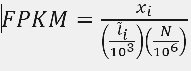
X = mapped reads count N = number of reads L = Length of transcripts
Featurecount output (Read count)
head -n 2 /data/gpfs/assoc/bch709-3/Course_materials/mouse/mouse_featurecount.txt
Sum of FPKM for 12WK_R6-2_Rep_1.bamAligned.sortedByCoord.out.bam
cat /data/gpfs/assoc/bch709-3/Course_materials/mouse/mouse_featurecount.txt | egrep -v Geneid | awk '{ sum+=$7} END {print sum}'
Call Python
python
X = 553

total_umber_Reads_mapped = 47414569

Length = 3634

fpkm = X*(1000/Length)*(1000000/total_umber_Reads_mapped)

fpkm
ten to the ninth power = 10**9
fpkm=X/(Number_Reads_mapped*Length)*10**9
fpkm
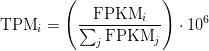
TPM
Transcripts Per Million
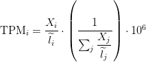
TPM calculation from reads count
cat /data/gpfs/assoc/bch709-3/Course_materials/mouse/mouse_featurecount.txt | egrep -v Geneid | awk '{ if($6 >= 0) sum+=$7/$6} END {print sum}'
sum_count_per_length=17352.8
X = 553
Length = 3634

TPM = (X/Length)*(1/sum_count_per_length )*10**6
Differential expression
DESeq2 edgeR (Neg-binom > GLM > Test) Limma-Voom (Neg-binom > Voom-transform > LM > Test)
DESeq
DESeq: This normalization method is included in the DESeq Bioconductor package (version 1.6.0) and is based on the hypothesis that most genes are not DE. A DESeq scaling factor for a given lane is computed as the median of the ratio, for each gene, of its read count over its geometric mean across all lanes. The underlying idea is that non-DE genes should have similar read counts across samples, leading to a ratio of 1. Assuming most genes are not DE, the median of this ratio for the lane provides an estimate of the correction factor that should be applied to all read counts of this lane to fulfill the hypothesis. By calling the estimateSizeFactors() and sizeFactors() functions in the DESeq Bioconductor package, this factor is computed for each lane, and raw read counts are divided by the factor associated with their sequencing lane.
DESeq2
EdgeR
Trimmed Mean of M-values (TMM): This normalization method is implemented in the edgeR Bioconductor package (version 2.4.0). It is also based on the hypothesis that most genes are not DE. The TMM factor is computed for each lane, with one lane being considered as a reference sample and the others as test samples. For each test sample, TMM is computed as the weighted mean of log ratios between this test and the reference, after exclusion of the most expressed genes and the genes with the largest log ratios. According to the hypothesis of low DE, this TMM should be close to 1. If it is not, its value provides an estimate of the correction factor that must be applied to the library sizes (and not the raw counts) in order to fulfill the hypothesis. The calcNormFactors() function in the edgeR Bioconductor package provides these scaling factors. To obtain normalized read counts, these normalization factors are re-scaled by the mean of the normalized library sizes. Normalized read counts are obtained by dividing raw read counts by these re-scaled normalization factors.
EdgeR
DESeq2 vs EdgeR Statistical tests for differential expression
DESeq2
DESeq2 uses raw counts, rather than normalized count data, and models the normalization to fit the counts within a Generalized Linear Model (GLM) of the negative binomial family with a logarithmic link. Statistical tests are then performed to assess differential expression, if any.
EdgeR
Data are normalized to account for sample size differences and variance among samples. The normalized count data are used to estimate per-gene fold changes and to perform statistical tests of whether each gene is likely to be differentially expressed.
EdgeR uses an exact test under a negative binomial distribution (Robinson and Smyth, 2008). The statistical test is related to Fisher’s exact test, though Fisher uses a different distribution.
DESeq2 vs EdgeR Normalization method
DESeq and EdgeR are very similar and both assume that no genes are differentially expressed. DEseq uses a “geometric” normalisation strategy, whereas EdgeR is a weighted mean of log ratios-based method. Both normalise data initially via the calculation of size / normalisation factors.
Negative binormal
DESeq2
ϕ was assumed to be a function of μ (population mean) determined by nonparametric regression. The recent version used in this paper follows a more versatile procedure. Firstly, for each transcript, an estimate of the dispersion is made, presumably using maximum likelihood. Secondly, the estimated dispersions for all transcripts are fitted to the functional form:
s
EdgeR
edgeR recommends a “tagwise dispersion” function, which estimates the dispersion on a gene-by-gene basis, and implements an empirical Bayes strategy for squeezing the estimated dispersions towards the common dispersion. Under the default setting, the degree of squeezing is adjusted to suit the number of biological replicates within each condition: more biological replicates will need to borrow less information from the complete set of transcripts and require less squeezing.
** DEseq uses a “geometric” normalisation strategy, whereas EdgeR is a weighted mean of log ratios-based method. Both normalise data initially via the calculation of size / normalisation factors **
DESEQ2
 The final step in the differential expression analysis workflow is fitting the raw counts to the negative binormal model and performing the statistical test for differentially expressed genes. In this step we essentially want to determine whether the mean expression levels of different sample groups are significantly different.
Differential expression analysis with DESeq2 involves multiple steps as displayed in the flowchart below in blue. Briefly, DESeq2 will model the raw counts, using normalization factors (size factors) to account for differences in library depth. Then, it will estimate the gene-wise dispersions and shrink these estimates to generate more accurate estimates of dispersion to model the counts. Finally, DESeq2 will fit the negative binomial model and perform hypothesis testing using the Wald test or Likelihood Ratio Test.

NOTE: DESeq2 is actively maintained by the developers and continuously being updated. As such, it is important that you note the version you are working with. Recently, there have been some rather big changes implemented that impact the output. To find out more detail about the specific modifications made to methods described in the original 2014 paper, take a look at this section in the DESeq2 vignette.
What is dispersion?
Dispersion is a measure of spread or variability in the data. Variance, standard deviation, IQR, among other measures, can all be used to measure dispersion. However, DESeq2 uses a specific measure of dispersion (α) related to the mean (μ) and variance of the data: Var = μ + α*μ^2. For genes with moderate to high count values, the square root of dispersion will be equal to the coefficient of variation (Var / μ). So 0.01 dispersion means 10% variation around the mean expected across biological replicates.
What does the DESeq2 dispersion represent?
The DESeq2 dispersion estimates are inversely related to the mean and directly related to variance. Based on this relationship, the dispersion is higher for small mean counts and lower for large mean counts. The dispersion estimates for genes with the same mean will differ only based on their variance. Therefore, the dispersion estimates reflect the variance in gene expression for a given mean value.
The plot of mean versus variance in count data below shows the variance in gene expression increases with the mean expression (each black dot is a gene). Notice that the relationship between mean and variance is linear on the log scale, and for higher means, we could predict the variance relatively accurately given the mean. However, for low mean counts, the variance estimates have a much larger spread; therefore, the dispersion estimates will differ much more between genes with small means.

How does the dispersion relate to our model?
To accurately model sequencing counts, we need to generate accurate estimates of within-group variation (variation between replicates of the same sample group) for each gene. With only a few (3-6) replicates per group, the estimates of variation for each gene are often unreliable (due to the large differences in dispersion for genes with similar means).
To address this problem, DESeq2 shares information across genes to generate more accurate estimates of variation based on the mean expression level of the gene using a method called ‘shrinkage’. DESeq2 assumes that genes with similar expression levels have similar dispersion.
Estimating the dispersion for each gene separately:
To model the dispersion based on expression level (mean counts of replicates), the dispersion for each gene is estimated using maximum likelihood estimation. In other words, given the count values of the replicates, the most likely estimate of dispersion is calculated.
Fit curve to gene-wise dispersion estimates
This curve is displayed as a red line in the figure below, which plots the estimate for the expected dispersion value for genes of a given expression strength. Each black dot is a gene with an associated mean expression level and maximum likelihood estimation (MLE) of the dispersion (Step 1).

The curve allows for more accurate identification of differentially expressed genes when sample sizes are small, and the strength of the shrinkage for each gene depends on :
- how close gene dispersions are from the curve
- sample size (more samples = less shrinkage)
This shrinkage method is particularly important to reduce false positives in the differential expression analysis. Genes with low dispersion estimates are shrunken towards the curve, and the more accurate, higher shrunken values are output for fitting of the model and differential expression testing.
Dispersion estimates that are slightly above the curve are also shrunk toward the curve for better dispersion estimation; however, genes with extremely high dispersion values are not. This is due to the likelihood that the gene does not follow the modeling assumptions and has higher variability than others for biological or technical reasons [1]. Shrinking the values toward the curve could result in false positives, so these values are not shrunken. These genes are shown surrounded by blue circles below.
Mouse DEG
Activate environment
conda activate BCH709_RNASeq
Copy Mouse featurecount results
cp /data/gpfs/assoc/bch709-3/Course_materials/mouse/mouse_featurecount.txt /data/gpfs/assoc/bch709-3/${USER}/mouse/readcount/
Clean sample name
cut -f1,7-  mouse_featurecount.txt |  egrep -v "#" | sed 's/\Aligned\.sortedByCoord\.out\.bam//g; s/\.bam//g' >> mouse_featurecount_only.cnt
cut -f1,6-  mouse_featurecount.txt |  egrep -v "#" | sed 's/\Aligned\.sortedByCoord\.out\.bam//g; s/\.bam//g' >> mouse_featurecount_length.cnt
Copy read count to DEG folder
cp /data/gpfs/assoc/bch709-3/${USER}/mouse/readcount/mouse_featurecount_* /data/gpfs/assoc/bch709-3/${USER}/mouse/DEG
Go to DEG folder
cd /data/gpfs/assoc/bch709-3/${USER}/mouse/DEG
sample files
cp /data/gpfs/assoc/bch709-3/Course_materials/mouse/mouse_sample_association /data/gpfs/assoc/bch709-3/${USER}/mouse/DEG

cp /data/gpfs/assoc/bch709-3/Course_materials/mouse/mouse_contrast /data/gpfs/assoc/bch709-3/${USER}/mouse/DEG

cd /data/gpfs/assoc/bch709-3/${USER}/mouse/DEG
PtR (Quality Check Your Samples and Biological Replicates)
Once you’ve performed transcript quantification for each of your biological replicates, it’s good to examine the data to ensure that your biological replicates are well correlated, and also to investigate relationships among your samples. If there are any obvious discrepancies among your sample and replicate relationships such as due to accidental mis-labeling of sample replicates, or strong outliers or batch effects, you’ll want to identify them before proceeding to subsequent data analyses (such as differential expression).
cd /data/gpfs/assoc/bch709-3/${USER}/mouse/DEG
PtR  --matrix mouse_featurecount_only.cnt  --samples mouse_sample_association --CPM  --log2 --min_rowSums 10   --sample_cor_matrix --compare_replicates
PtR download on local
scp [YOURID]@pronghorn.rc.unr.edu:/data/gpfs/assoc/bch709-3/[YOURID]/mouse/DEG/*.pdf .
If this is not working on local Mac
echo "setopt nonomatch" >> ~/.zshrc
DEG analysis on Pronghorn
cd /data/gpfs/assoc/bch709-3/${USER}/mouse/DEG

run_DE_analysis.pl --matrix mouse_featurecount_only.cnt --method DESeq2 --samples_file mouse_sample_association --contrasts mouse_contrast --output mouse_rnaseq
DEG analysis results
ls mouse_rnaseq
TPM/FPKM calculation
python /data/gpfs/assoc/bch709-3/Course_materials/script/tpm_raw_exp_calculator.py -count mouse_featurecount_length.cnt
TPM and FPKM calculation output
mouse_featurecount_length.cnt.fpkm.xls
mouse_featurecount_length.cnt.fpkm.tab
mouse_featurecount_length.cnt.tpm.xls
mouse_featurecount_length.cnt.tpm.tab
DEG subset
cd /data/gpfs/assoc/bch709-3/${USER}/mouse/DEG/mouse_rnaseq
analyze_diff_expr.pl --samples /data/gpfs/assoc/bch709-3/${USER}/mouse/DEG/mouse_sample_association  --matrix /data/gpfs/assoc/bch709-3/${USER}/mouse/DEG/mouse_featurecount_length.cnt.tpm.tab -P 0.01 -C 2 --output mouse_RNASEQ_P001_C2
analyze_diff_expr.pl --samples /data/gpfs/assoc/bch709-3/${USER}/mouse/DEG/mouse_sample_association  --matrix /data/gpfs/assoc/bch709-3/${USER}/mouse/DEG/mouse_featurecount_length.cnt.tpm.tab -P 0.01 -C 1 --output mouse_RNASEQ_P001_C1
DEG download
scp -r [YOURID]@pronghorn.rc.unr.edu:/data/gpfs/assoc/bch709-3/wyim/mouse/DEG/ .
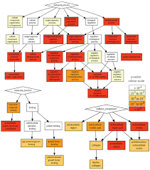
Functional analysis • GO
Gene enrichment analysis (Hypergeometric test) Gene set enrichment analysis (GSEA) Gene ontology / Reactome databases
Gene Ontology
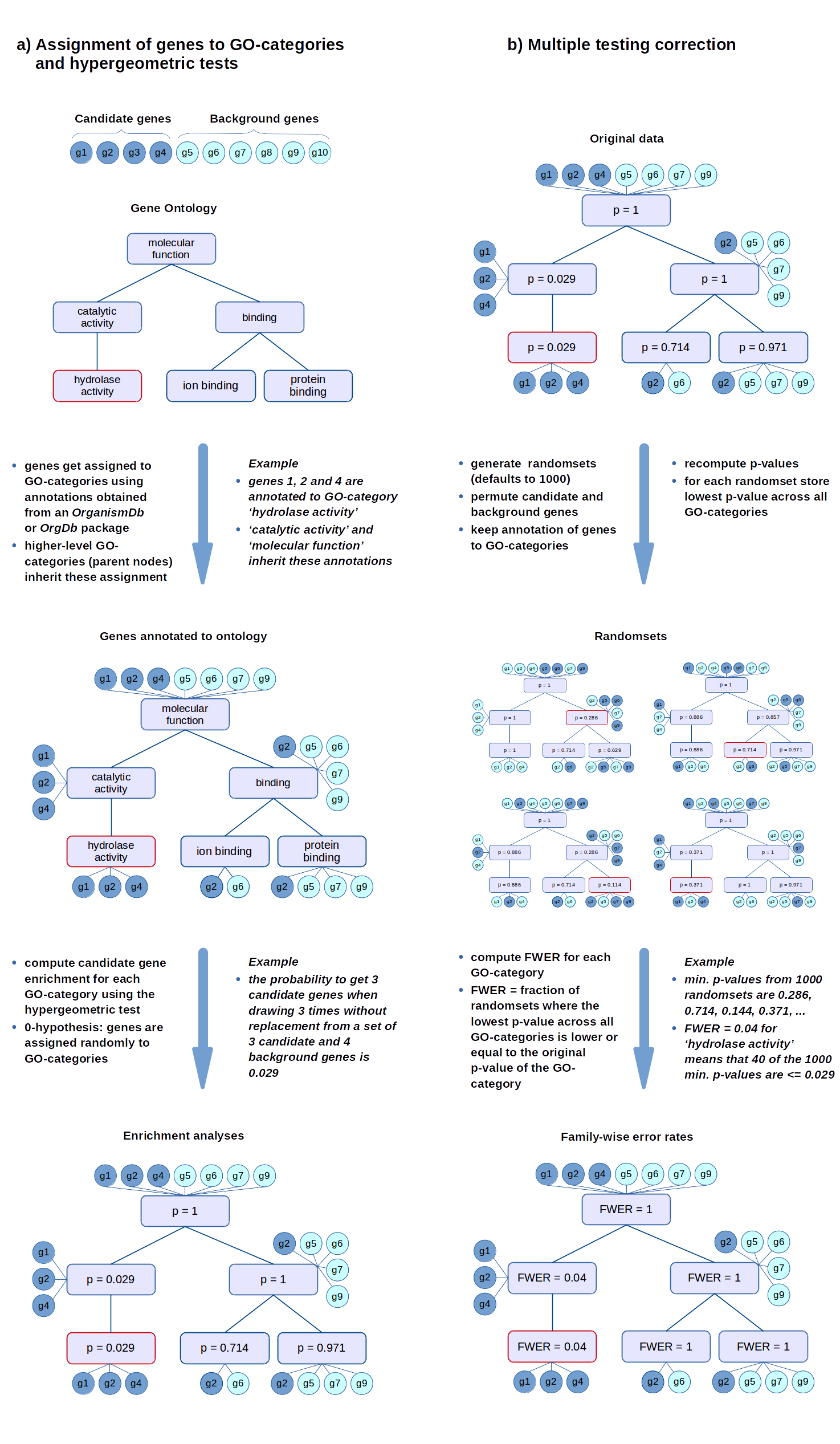
Gene Ontology project is a major bioinformatics initiative Gene ontology is an annotation system The project provides the controlled and consistent vocabulary of terms and gene product annotations, i.e. terms occur only once, and there is a dictionary of allowed words GO describes how gene products behave in a cellular context A consistent description of gene products attributes in terms of their associated biological processes, cellular components and molecular functions in a species-independent manner Each GO term consists of a unique alphanumerical identifier, a common name, synonyms (if applicable), and a definition Each term is assigned to one of the three ontologies Terms have a textual definition When a term has multiple meanings depending on species, the GO uses a “sensu” tag to differentiate among them (trichome differentiation (sensu Magnoliophyta)
hypergeometric test
The hypergeometric distribution is the lesser-known cousin of the binomial distribution, which describes the probability of k successes in n draws with replacement. The hypergeometric distribution describes probabilities of drawing marbles from the jar without putting them back in the jar after each draw. The hypergeometric probability mass function is given by (using the original variable convention)

FWER
The FWER for the other tests is computed in the same way: the gene-associated variables (scores or counts) are permuted while the annotations of genes to GO-categories stay fixed. Then the statistical tests are evaluated again for every GO-category.
Hypergeometric Test Example 1
Suppose we randomly select 2 cards without replacement from an ordinary deck of playing cards. What is the probability of getting exactly 2 cards you want (i.e., Ace or 10)?
Solution: This is a hypergeometric experiment in which we know the following:
N = 52; since there are 52 cards in a deck. k = 16; since there are 16 Ace or 10 cards in a deck. n = 2; since we randomly select cards from the deck. x = 2; since 2 of the cards we select are red. We plug these values into the hypergeometric formula as follows:
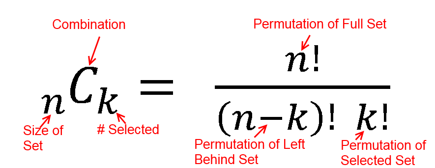
h(x; N, n, k) = [ kCx ] [ N-kCn-x ] / [ NCn ]
h(2; 52, 2, 16) = [ 16C2 ] [ 48C1 ] / [ 52C2 ]
h(2; 52, 2, 16) = [ 325 ] [ 1 ] / [ 1,326 ]
h(2; 52, 2, 16) = 0.0904977
Thus, the probability of randomly selecting 2 Ace or 10 cards is 9%
| category | probability |
|---|---|
| probability mass f | 0.09049773755656108597285 |
| lower cumulative P | 1 |
| upper cumulative Q | 0.09049773755656108597285 |
| Expectation | 0.6153846153846153846154 |
Hypergeometric Test Example 2
Suppose we have 30 DEGs in human genome (200). What is the probability of getting 10 oncogene?
An oncogene is a gene that has the potential to cause cancer.
Solution: This is a hypergeometric experiment in which we know the following:
N = 200; since there are 200 genes in human genome k = 10; since there are 10 oncogenes in human n = 30; since 30 DEGs x = 5; since 5 of the oncogenes in DEGs.
We plug these values into the hypergeometric formula as follows:
h(x; N, n, k) = [ kCx ] [ N-kCn-x ] / [ NCn ]
h(5; 200, 30, 10) = [ 10C5 ] [ 190C25 ] / [ 200C30 ]
h(5; 200, 30, 10) = [ 252 ] [ 11506192278177947613740456466942 ] / [ 409681705022127773530866523638950880 ]
h(5; 200, 30, 10) = 0.007078
Thus, the probability of oncogene 0.7%.
hypergeometry.png
hypergeometric distribution value
| category | probability |
|---|---|
| probability mass f | 0.0070775932109153651831923063371216961166297 |
| lower cumulative P | 0.99903494867072865323201131115533112651846 |
| upper cumulative Q | 0.0080426445401867119511809951817905695981658 |
| Expectation | 1.5 |
False Discovery Rate (FDR) q-value
The false discovery rate (FDR) is a method of conceptualizing the rate of type I errors in null hypothesis testing when conducting multiple comparisons. FDR-controlling procedures are designed to control the expected proportion of “discoveries” (rejected null hypotheses) that are false (incorrect rejections).
- Benjamini–Yekutieli
- Benjamini–Hochberg
- Bonferroni-Selected–Bonferroni
- Bonferroni and Sidak
REViGO
http://revigo.irb.hr/revigo.jsp
cleverGO
http://www.tartaglialab.com/GO_analyser/tutorial
MetaScape
http://metascape.org/gp/index.html
DAVID
https://david.ncifcrf.gov/
Araport
http://araport.org
Paper read
Fu, Yu, et al. “Elimination of PCR duplicates in RNA-seq and small RNA-seq using unique molecular identifiers.” BMC genomics 19.1 (2018): 531 Parekh, Swati, et al. “The impact of amplification on differential expression analyses by RNA-seq.” Scientific reports 6 (2016): 25533 Klepikova, Anna V., et al. “Effect of method of deduplication on estimation of differential gene expression using RNA-seq.” PeerJ 5 (2017): e3091