Metrics
- Number of contigs
- Average contig length
- Median contig length
- Maximum contig length
- “N50”, “NG50”, “D50”
N50

N50 example
| Contig Length | Cumulative Sum |
|---|---|
| 100 | 100 |
| 200 | 300 |
| 230 | 530 |
| 400 | 930 |
| 750 | 1680 |
| 852 | 2532 |
| 950 | 3482 |
| 990 | 4472 |
| 1020 | 5492 |
| 1278 | 6770 |
| 1280 | 8050 |
| 1290 | 9340 |
Check Genome Size by Illumina Reads
cd /data/gpfs/assoc/bch709-1/<YOUR_ID>/
mkdir -p Genome_assembly/Illumina
cd Genome_assembly/Illumina
Create Preprocessing Env
conda create -n preprocessing python=3 -y

conda activate preprocessing

conda install -c bioconda trim-galore jellyfish=2.2.10 'multiqc<1.34' nanostat nanoplot -y
Reads Download
https://www.dropbox.com/s/ax38m9wra44lsgi/WGS_R1.fq.gz
https://www.dropbox.com/s/kp7et2du5c2v385/WGS_R2.fq.gz
Count Reads Number in file
echo $(zcat WGS_R1.fq.gz |wc -l)/4 | bc

echo $(cat WGS_R1.fq |wc -l)/4 | bc
Advanced approach
for i in `ls -1 *.fq.gz`; do echo $(zcat ${i} | wc -l)/4|bc; done


***For all gzip compressed fastq files, display the number of reads since 4 lines = 1 reads***
Reads Trimming
#!/bin/bash
#SBATCH --job-name=Trim
#SBATCH --cpus-per-task=8
#SBATCH --time=2:00:00
#SBATCH --mem=30g
#SBATCH --account=cpu-s2-bch709-1
#SBATCH --partition=cpu-s2-core-0
#SBATCH --mail-type=all
#SBATCH --mail-user=<YOUR ID>@unr.edu

trim_galore --paired   --three_prime_clip_R1 10 --three_prime_clip_R2 10 --cores 8  --max_n 40  -o trimmed_fastq --fastqc <READ_R1> <READ_R2>

multiqc . -n WGS_Illumina --exclude rsem --exclude gatk
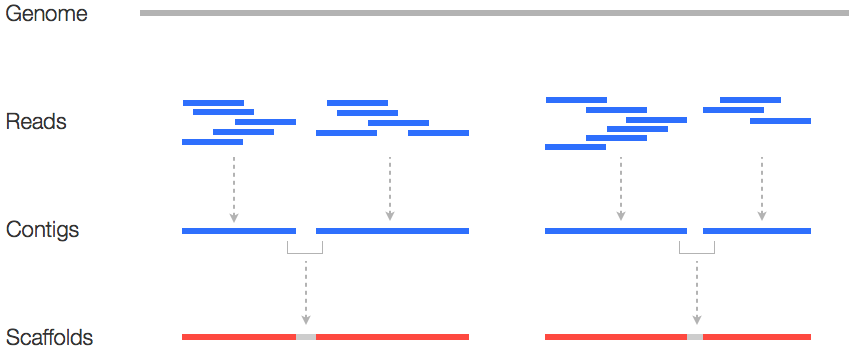
Why assemble genomes
- Produce a reference for new species
- Genomic variation can be studied by comparing against the reference
- A wide variety of molecular biological tools become available or more effective
- Coding sequences can be studied in the context of their related non-coding (eg regulatory) sequences
- High level genome structure (number, arrangement of genes and repeats) can be studied
Assembly is very challenging (“impossible”) because
- Sequencing bias under represents certain regions
- Reads are short relative to genome size
- Repeats create tangled hubs in the assembly graph
- Sequencing errors cause detours and bubbles in the assembly graph
Prerequisite
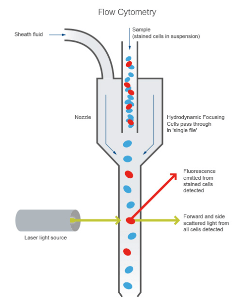
Flow Cytometry
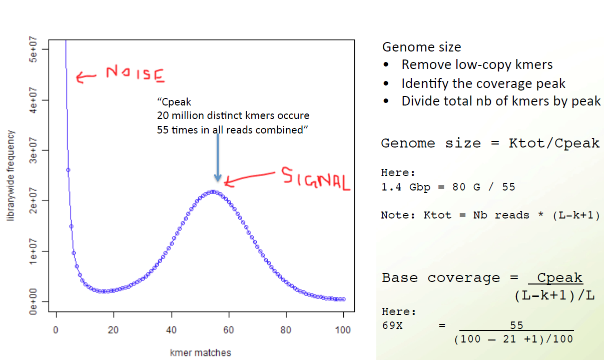
K-mer spectrum
K-mer counting
mkdir kmer && cd kmer
#!/bin/bash
#SBATCH --job-name=Trim
#SBATCH --cpus-per-task=10
#SBATCH --time=2:00:00
#SBATCH --mem=10g
#SBATCH --account=cpu-s2-bch709-1
#SBATCH --partition=cpu-s2-core-0
#SBATCH --mail-type=all
#SBATCH --mail-user=<YOUR ID>@unr.edu
#SBATCH -o trim.out # STDOUT
#SBATCH -e trim.err # STDERR
jellyfish count -C -m 21 -s 100000000 -t 10  -o reads.jf <(zcat ../trimmed_fastq/*.gz)
jellyfish histo -t 10 reads.jf > reads_jf.histo
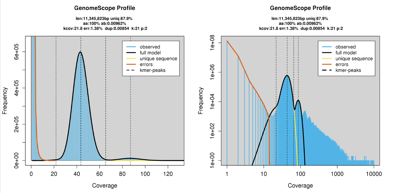
Upload to GenomeScope
http://qb.cshl.edu/genomescope/genomescope2.0
Genome assembly Spades
cd /data/gpfs/assoc/bch709-1/<YOURID>/Genome_assembly/Illumina/
mkdir Spades
cd Spades
conda create -n genomeassembly -y
conda activate genomeassembly
conda install -c bioconda spades canu pacbio_falcon samtools minimap2 'multiqc<1.34'  openssl=1.0 -y
conda install -c r r-ggplot2 r-stringr r-scales r-argparse -y
#!/bin/bash
#SBATCH --job-name=Spades
#SBATCH --cpus-per-task=32
#SBATCH --time=2:00:00
#SBATCH --mem=64g
#SBATCH --account=cpu-s2-bch709-1
#SBATCH --partition=cpu-s2-core-0
#SBATCH --mail-type=all
#SBATCH --mail-user=<YOUR ID>@unr.edu
#SBATCH -o Spades.out # STDOUT
#SBATCH -e Spades.err # STDERR

spades.py -k 21,33,55,77 --careful -1 <trim_galore output> -2 <trim_galore output> -o spades_output --memory 64 --threads 32
###Spade
Log
Command line: /data/gpfs/home/wyim/miniconda3/envs/genomeassembly/bin/spades.py -k21,33,55,77     --careful       -1      /data/gpfs/assoc/bch709-1/wyim/gee/trimmed_fastq/WGS_R1_val_1.fq.gz    -2      /data/gpfs/assoc/bch709-1/wyim/gee/trimmed_fastq/WGS_R2_val_2.fq.gz    -o      /data/gpfs/assoc/bch709-1/wyim/gee/spades_output       --memory        120     --threads       32

System information:
  SPAdes version: 3.13.1
  Python version: 3.7.3
  OS: Linux-3.10.0-957.27.2.el7.x86_64-x86_64-with-centos-7.6.1810-Core

Output dir: /data/gpfs/assoc/bch709-1/wyim/gee/spades_output
Mode: read error correction and assembling
Debug mode is turned OFF

Dataset parameters:
  Multi-cell mode (you should set '--sc' flag if input data was obtained with MDA (single-cell) technology or --meta flag if processing metagenomic dataset)
  Reads:
    Library number: 1, library type: paired-end
      orientation: fr
      left reads: ['/data/gpfs/assoc/bch709-1/wyim/gee/trimmed_fastq/WGS_R1_val_1.fq.gz']
      right reads: ['/data/gpfs/assoc/bch709-1/wyim/gee/trimmed_fastq/WGS_R2_val_2.fq.gz']
      interlaced reads: not specified
      single reads: not specified
      merged reads: not specified
Read error correction parameters:
  Iterations: 1
  PHRED offset will be auto-detected
  Corrected reads will be compressed
Assembly parameters:
  k: [21, 33, 55, 77]
  Repeat resolution is enabled
  Mismatch careful mode is turned ON
  MismatchCorrector will be used
  Coverage cutoff is turned OFF
Other parameters:
  Dir for temp files: /data/gpfs/assoc/bch709-1/wyim/gee/spades_output/tmp
  Threads: 64
  Memory limit (in Gb): 140


======= SPAdes pipeline started. Log can be found here: /data/gpfs/assoc/bch709-1/wyim/gee/spades_output/spades.log


===== Read error correction started.


== Running read error correction tool: /data/gpfs/home/wyim/miniconda3/envs/genomeassembly/bin/spades-hammer /data/gpfs/assoc/bch709-1/wyim/gee/spades_output/corrected/configs/config.info

  0:00:00.000     4M / 4M    INFO    General                 (main.cpp                  :  75)   Starting BayesHammer, built from N/A, git revision N/A
  0:00:00.000     4M / 4M    INFO    General                 (main.cpp                  :  76)   Loading config from /data/gpfs/assoc/bch709-1/wyim/gee/spades_output/corrected/configs/config.info
  0:00:00.001     4M / 4M    INFO    General                 (main.cpp                  :  78)   Maximum # of threads to use (adjusted due to OMP capabilities): 32
  0:00:00.001     4M / 4M    INFO    General                 (memory_limit.cpp          :  49)   Memory limit set to 140 Gb
  0:00:00.001     4M / 4M    INFO    General                 (main.cpp                  :  86)   Trying to determine PHRED offset
  0:00:00.038     4M / 4M    INFO    General                 (main.cpp                  :  92)   Determined value is 33
  0:00:00.038     4M / 4M    INFO    General                 (hammer_tools.cpp          :  36)   Hamming graph threshold tau=1, k=21, subkmer positions = [ 0 10 ]
  0:00:00.038     4M / 4M    INFO    General                 (main.cpp                  : 113)   Size of aux. kmer data 24 bytes
     === ITERATION 0 begins ===
  0:00:00.042     4M / 4M    INFO   K-mer Index Building     (kmer_index_builder.hpp    : 301)   Building kmer index
  0:00:00.042     4M / 4M    INFO    General                 (kmer_index_builder.hpp    : 117)   Splitting kmer instances into 512 files using 32 threads. This might take a while.
  0:00:00.043     4M / 4M    INFO    General                 (file_limit.hpp            :  32)   Open file limit set to 65536
  0:00:00.043     4M / 4M    INFO    General                 (kmer_splitters.hpp        :  89)   Memory available for splitting buffers: 1.45829 Gb
  0:00:00.043     4M / 4M    INFO    General                 (kmer_splitters.hpp        :  97)   Using cell size of 131072
  0:00:02.300    17G / 17G   INFO   K-mer Splitting          (kmer_data.cpp             :  97)   Processing /data/gpfs/assoc/bch709-1/wyim/gee/trimmed_fastq/WGS_R1_val_1.fq.gz
  0:00:19.373    17G / 18G   INFO   K-mer Splitting          (kmer_data.cpp             : 107)   Processed 3022711 reads
  0:00:19.373    17G / 18G   INFO   K-mer Splitting          (kmer_data.cpp             :  97)   Processing /data/gpfs/assoc/bch709-1/wyim/gee/trimmed_fastq/WGS_R2_val_2.fq.gz
  0:00:37.483    17G / 18G   INFO   K-mer Splitting          (kmer_data.cpp             : 107)   Processed 6045422 reads
  0:00:37.483    17G / 18G   INFO   K-mer Splitting          (kmer_data.cpp             : 112)   Total 6045422 reads processed
  0:00:39.173   128M / 18G   INFO    General                 (kmer_index_builder.hpp    : 120)   Starting k-mer counting.
  0:00:43.628   128M / 18G   INFO    General                 (kmer_index_builder.hpp    : 127)   K-mer counting done. There are 318799406 kmers in total.
  0:00:43.628   128M / 18G   INFO    General                 (kmer_index_builder.hpp    : 133)   Merging temporary buckets.
  0:00:48.548   128M / 18G   INFO   K-mer Index Building     (kmer_index_builder.hpp    : 314)   Building perfect hash indices
  0:00:58.437   320M / 18G   INFO    General                 (kmer_index_builder.hpp    : 150)   Merging final buckets.
  0:01:00.516   320M / 18G   INFO   K-mer Index Building     (kmer_index_builder.hpp    : 336)   Index built. Total 147835808 bytes occupied (3.70981 bits per kmer).
  0:01:00.518   320M / 18G   INFO   K-mer Counting           (kmer_data.cpp             : 356)   Arranging kmers in hash map order
  0:02:50.247     5G / 18G   INFO    General                 (main.cpp                  : 148)   Clustering Hamming graph.
  0:05:15.609     5G / 18G   INFO    General                 (main.cpp                  : 155)   Extracting clusters
  0:06:20.894     5G / 18G   INFO    General                 (main.cpp                  : 167)   Clustering done. Total clusters: 47999941
  0:06:20.900     2G / 18G   INFO   K-mer Counting           (kmer_data.cpp             : 376)   Collecting K-mer information, this takes a while.
  0:06:23.367     9G / 18G   INFO   K-mer Counting           (kmer_data.cpp             : 382)   Processing /data/gpfs/assoc/bch709-1/wyim/gee/trimmed_fastq/WGS_R1_val_1.fq.gz
  0:06:41.328     9G / 18G   INFO   K-mer Counting           (kmer_data.cpp             : 382)   Processing /data/gpfs/assoc/bch709-1/wyim/gee/trimmed_fastq/WGS_R2_val_2.fq.gz
  0:06:59.453     9G / 18G   INFO   K-mer Counting           (kmer_data.cpp             : 389)   Collection done, postprocessing.
  0:07:00.669     9G / 18G   INFO   K-mer Counting           (kmer_data.cpp             : 403)   There are 318799406 kmers in total. Among them 268145204 (84.1109%) are singletons.
  0:07:00.669     9G / 18G   INFO    General                 (main.cpp                  : 173)   Subclustering Hamming graph
  0:15:33.177     9G / 18G   INFO   Hamming Subclustering    (kmer_cluster.cpp          : 649)   Subclustering done. Total 11739 non-read kmers were generated.
  0:15:33.177     9G / 18G   INFO   Hamming Subclustering    (kmer_cluster.cpp          : 650)   Subclustering statistics:
  0:15:33.177     9G / 18G   INFO   Hamming Subclustering    (kmer_cluster.cpp          : 651)     Total singleton hamming clusters: 31640728. Among them 6970 (0.0220286%) are good
  0:15:33.177     9G / 18G   INFO   Hamming Subclustering    (kmer_cluster.cpp          : 652)     Total singleton subclusters: 14379. Among them 2710 (18.8469%) are good
  0:15:33.177     9G / 18G   INFO   Hamming Subclustering    (kmer_cluster.cpp          : 653)     Total non-singleton subcluster centers: 20505272. Among them 19729791 (96.2181%) are good
  0:15:33.177     9G / 18G   INFO   Hamming Subclustering    (kmer_cluster.cpp          : 654)     Average size of non-trivial subcluster: 14.0052 kmers
  0:15:33.177     9G / 18G   INFO   Hamming Subclustering    (kmer_cluster.cpp          : 655)     Average number of sub-clusters per non-singleton cluster: 1.25432  0:15:33.177     9G / 18G   INFO   Hamming Subclustering    (kmer_cluster.cpp          : 656)     Total solid k-mers: 19739471
  0:15:33.177     9G / 18G   INFO   Hamming Subclustering    (kmer_cluster.cpp          : 657)     Substitution probabilities: [4,4]((0.944751,0.0179573,0.0182179,0.0190737),(0.0183827,0.9447,0.0178155,0.0191018),(0.0189441,0.0177016,0.94483,0.0185242),(0.0190054,0.0181679,0.0179184,0.944908))
  0:15:33.233     9G / 18G   INFO    General                 (main.cpp                  : 178)   Finished clustering.
  0:15:33.233     9G / 18G   INFO    General                 (main.cpp                  : 197)   Starting solid k-mers expansion in 32 threads.
  0:16:01.042     9G / 18G   INFO    General                 (main.cpp                  : 218)   Solid k-mers iteration 0 produced 1807215 new k-mers.
  0:16:28.728     9G / 18G   INFO    General                 (main.cpp                  : 218)   Solid k-mers iteration 1 produced 152036 new k-mers.
  0:16:56.455     9G / 18G   INFO    General                 (main.cpp                  : 218)   Solid k-mers iteration 2 produced 13249 new k-mers.
  0:17:24.110     9G / 18G   INFO    General                 (main.cpp                  : 218)   Solid k-mers iteration 3 produced 1204 new k-mers.
  0:17:51.837     9G / 18G   INFO    General                 (main.cpp                  : 218)   Solid k-mers iteration 4 produced 93 new k-mers.
  0:18:19.634     9G / 18G   INFO    General                 (main.cpp                  : 218)   Solid k-mers iteration 5 produced 20 new k-mers.
  0:18:47.540     9G / 18G   INFO    General                 (main.cpp                  : 218)   Solid k-mers iteration 6 produced 7 new k-mers.
  0:18:47.540     9G / 18G   INFO    General                 (main.cpp                  : 222)   Solid k-mers finalized
  0:18:47.540     9G / 18G   INFO    General                 (hammer_tools.cpp          : 220)   Starting read correction in 32 threads.
  0:18:47.540     9G / 18G   INFO    General                 (hammer_tools.cpp          : 233)   Correcting pair of reads: /data/gpfs/assoc/bch709-1/wyim/gee/trimmed_fastq/WGS_R1_val_1.fq.gz and /data/gpfs/assoc/bch709-1/wyim/gee/trimmed_fastq/WGS_R2_val_2.fq.gz
  0:19:07.696    12G / 18G   INFO    General                 (hammer_tools.cpp          : 168)   Prepared batch 0 of 3022711 reads.
  0:19:28.112    12G / 18G   INFO    General                 (hammer_tools.cpp          : 175)   Processed batch 0
  0:19:33.861    12G / 18G   INFO    General                 (hammer_tools.cpp          : 185)   Written batch 0
  0:19:35.020     9G / 18G   INFO    General                 (hammer_tools.cpp          : 274)   Correction done. Changed 10322067 bases in 4896755 reads.
  0:19:35.020     9G / 18G   INFO    General                 (hammer_tools.cpp          : 275)   Failed to correct 299 bases out of 782307432.
  0:19:35.053   128M / 18G   INFO    General                 (main.cpp                  : 255)   Saving corrected dataset description to /data/gpfs/assoc/bch709-1/wyim/gee/spades_output/corrected/corrected.yaml
  0:19:35.054   128M / 18G   INFO    General                 (main.cpp                  : 262)   All done. Exiting.

== Compressing corrected reads (with pigz)

== Dataset description file was created: /data/gpfs/assoc/bch709-1/wyim/gee/spades_output/corrected/corrected.yaml


===== Read error correction finished.


===== Assembling started.


===== Mismatch correction finished.

 * Corrected reads are in /data/gpfs/assoc/bch709-1/wyim/gee/spades_output/corrected/
 * Assembled contigs are in /data/gpfs/assoc/bch709-1/wyim/gee/spades_output/contigs.fasta
 * Assembled scaffolds are in /data/gpfs/assoc/bch709-1/wyim/gee/spades_output/scaffolds.fasta
 * Paths in the assembly graph corresponding to the contigs are in /data/gpfs/assoc/bch709-1/wyim/gee/spades_output/contigs.paths
 * Paths in the assembly graph corresponding to the scaffolds are in /data/gpfs/assoc/bch709-1/wyim/gee/spades_output/scaffolds.paths
 * Assembly graph is in /data/gpfs/assoc/bch709-1/wyim/gee/spades_output/assembly_graph.fastg
 * Assembly graph in GFA format is in /data/gpfs/assoc/bch709-1/wyim/gee/spades_output/assembly_graph_with_scaffolds.gfa

======= SPAdes pipeline finished.

SPAdes log can be found here: /data/gpfs/assoc/bch709-1/wyim/gee/spades_output/spades.log

Thank you for using SPAdes!
Assembly statistics
N50 example
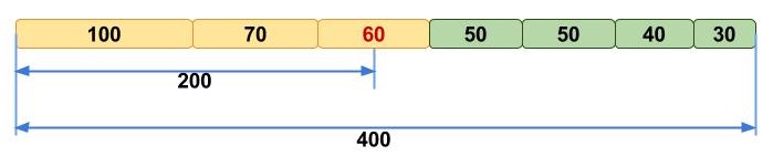
N50 is a measure to describe the quality of assembled genomes that are fragmented in contigs of different length. The N50 is defined as the minimum contig length needed to cover 50% of the genome.
| Contig Length |
|---|
| 100 |
| 200 |
| 230 |
| 400 |
| 750 |
| 852 |
| 950 |
| 990 |
| 1020 |
| 1278 |
| 1280 |
| 1290 |
conda install -c bioconda -c conda-forge assembly-stats
cd spades_output
assembly-stats scaffolds.fasta
assembly-stats contigs.fasta
Assembly statistics result
stats for scaffolds.fasta
sum = 11241648, n = 2345, ave = 4793.88, largest = 677246
N50 = 167555, n = 17
N60 = 124056, n = 24
N70 = 97565, n = 34
N80 = 72177, n = 48
N90 = 38001, n = 68
N100 = 78, n = 2345
N_count = 308
Gaps = 4
stats for contigs.fasta
sum = 11241391, n = 2349, ave = 4785.61, largest = 666314
N50 = 167555, n = 17
N60 = 123051, n = 25
N70 = 95026, n = 36
N80 = 70916, n = 50
N90 = 36771, n = 71
N100 = 78, n = 2349
N_count = 0
Gaps = 0
cat scaffolds.paths
NODE_1_length_677246_cov_27.741934
5330914+,39250+,5099246-;
4754344-,4601428-,5180688-,1424894+,5327688+,732820-,5237058-,5052460-,4723018+,4800852+,5331930-,732820-,5019006-,5052460-,4755300-,4800852+,5331932-,5060558+,5185654-,5071338-,5178452+,5178460+,5178468+,5178476+,5254862-,5325448+,88806-,5243982-,5053698+,1425522-,5239940+,5238056-,4867204-,5331654+
NODE_1_length_677246_cov_27.741934'
5331654-,4867204+,5238056+,5239940-,1425522+,5053698-,5243982+,88806+,5325448-,5254862+,5178476-,5178468-,5178460-,5178452-,5071338+,5185654+,5060558-,5331932+,4800852-,4755300+,5052460+,5019006+,732820+,5331930+,4800852-,4723018-,5052460+,5237058+,732820+,5327688-,1424894-,5180688+,4601428+,4754344+;
5099246+,39250-,5330914-
NODE_2_length_666314_cov_27.644287
5327204+,103640+,4836832-,4851626+,5361530-,5361524-,5361528-,5329856-,1126012-,5329854-,1126012-,5236812+,5052228+,5236810+,5052228+,5099424-,4479150+,4812968+,4479150+,5062132+,414588+,5051858+,414588+,5331378+,4760742-,4925978+,5327370-,474724-,5094420-,4653402-,5331664-,4961012-,5018412+,5072166+,5040312+,5030606-,4961012-,5236106+,5072166+,5072168+,4915570-,5050466-,4765966-,5059218-,4915570-,5058386-,5236104+,5095538-,5095540-,5095538-,5149466+,4774822-,5017666+,4774822-,5065186-,876886-,4799048-,876886-,5332178-
NODE_2_length_666314_cov_27.644287'
5332178+,876886+,4799048+,876886+,5065186+,4774822+,5017666-,4774822+,5149466-,5095538+,5095540+,5095538+,5236104-,5058386+,4915570+,5059218+,4765966+,5050466+,4915570+,5072168-,5072166-,5236106-,4961012+,5030606+,5040312-,5072166-,5018412-,4961012+,5331664+,4653402+,5094420+,474724+,5327370+,4925978-,4760742+,5331378-,414588-,5051858-,414588-,5062132-,4479150-,4812968-,4479150-,5099424+,5052228-,5236810-,5052228-,5236812-,1126012+,5329854+,1126012+,5329856+,5361528+,5361524+,5361530+,4851626-,4836832+,103640-,5327204-
NODE_3_length_613985_cov_27.733595
5250014-,5121298+,5057128-,4953418-,5238246+,5264238+,5264242+,4468126+,5331520+,4813546-,4676908-,4813546-,5059540-,4862238+,5032536-,4862238+,5045932+,1122610+,4827200-,928516+,5031788-,4629584+,5007546-,1271448+,4907228+,1271448+,5099418-,5331326-,5030236-,5236282-,5100426-,5100418-,5100430-,139162-,4675324-,5354642-,372-,374+,5044194+,5058512+,5325918+,4544022-,4816684-,427838+,5238146+,269904+,117192-
NODE_3_length_613985_cov_27.733595'
117192+,269904-,5238146-,427838-,4816684+,4544022+,5325918-,5058512-,5044194-,374-,372+,5354642+,4675324+,139162+,5100430+,5100418+,5100426+,5236282+,5030236+,5331326+,5099418+,1271448-,4907228-,1271448-,5007546+,4629584-,5031788+,928516-,4827200+,1122610-,5045932-,4862238-,5032536+,4862238-,5059540+,4813546+,4676908+,4813546+,5331520-,4468126-,5264242-,5264238-,5238246-,4953418+,5057128+,5121298-,5250014+
NODE_4_length_431556_cov_27.699452
FASTG file format
>EDGE_5360468_length_246_cov_13.568047:EDGE_5284398_length_327_cov_11.636000,EDGE_5354800_length_230_cov_14.470588';
GCTTCTTCTTGCTTCTCAAAGCTTTGTTGGTTTAGCCAAAGTCCAGATGAGTCTTTATCT
TTGTATCTTCTAACAAGGAAACACTACTTAGGCTTTTAGGATAAGCTTGCGGTTTAAGTT
TGTATACTCAATCATACACATGACATCAAGTCATATTCGACTCCAAAACACTAACCAAGC
TTCTTCTTGCACCTCAAAGCTTTGTTGGTTTAGCCAAAGTCCATATAAGTCTTTGTCTTT
GTATCT
>EDGE_5360470_length_161_cov_15.607143:EDGE_5332762_length_98_cov_43.619048';
GCTTCTTCTTGCTTCTCAAAGCTTTGTTGGTTTAGCCAAAGTCCAGATGAGTCTTTATCT
TTGTATCTTCTAACAAGAAAACACTACTTACGCTTTTAGGATAATGTTGCGGTTTAAGTT
CTTATACTCAATCATACACATGACATCAAGTCATATTCGAC
>EDGE_5354230_length_92_cov_267.066667':EDGE_5354222_length_86_cov_252.444444',EDGE_5355724_length_1189_cov_26.724820;
AAGCAAAGACTAAGTTTGGGGGAGTTGATAAGTGTGTATTTTGCATGTTTTGAGCATCCA
TTTGTCATCACTTTAGCATCATATCATCACTG
>EDGE_5344586_length_373_cov_22.574324:EDGE_5360654_length_82_cov_117.400000';
GCTAAAGTGATGACAAATGGATGCTCAAAACATGCAAAATACACACTTATCAACTCCCCC
AAACTTAGTCTTTGCTTAAGAACAAGCTGGAGGTGAGGTTTGAAAGCGGGGACTCAGAGC
CAAAGCAGCAGATAAACCAGATGAAATCAATGTCCAAGTTGATAGTTCTAAGTTGCGATA
TGATCGAATTCTACTCAAAAACGTTAGCCATGCCTTTTTATCAATCAATCCGACTCATAT
GCTCGACCTACACGTGTTTTCAAATCTACCAATCCCTTTAACATTCATTAGCTCTAGAAC
GTGAATCAAGCAATGCATCATCAATGAACTCATTTGGCTAAGGTAAAAGGTCAAGAGACA
AAGATGGTCCCTT
>EDGE_5354236_length_91_cov_242.857143:EDGE_5350728_length_80_cov_275.666667';
GCTAAAGTGATGACAAATGGATGCTCAAAACATGCAAAATACACACTTATCAACTCCCCC
AAACTTAGTCTTTGCTTGCCCTCAAGCAAAC
Genome assembly Spades
cd /data/gpfs/assoc/bch709-1/<YOURID>/Genome_assembly/Illumina/
mkdir Spades
cd Spades
conda create -n genomeassembly -y
conda activate genomeassembly
conda install  -c r -c conda-forge -c anaconda -c bioconda  spades canu pacbio_falcon samtools minimap2 'multiqc<1.34' openssl=1.0 -y
conda install  -c r -c conda-forge -c anaconda -c bioconda  r-ggplot2 r-stringr r-scales r-argparse -y
#!/bin/bash
#SBATCH --job-name=Spades
#SBATCH --cpus-per-task=32
#SBATCH --time=2:00:00
#SBATCH --mem=64g
#SBATCH --account=cpu-s2-bch709-1
#SBATCH --partition=cpu-s2-core-0
#SBATCH --mail-type=all
#SBATCH --mail-user=<YOUR ID>@unr.edu
#SBATCH -o Spades.out # STDOUT
#SBATCH -e Spades.err # STDERR

spades.py -k 21,33,55,77 --careful -1 <trim_galore output> -2 <trim_galore output> -o spades_output --memory 64 --threads 32
Spade
Log
Command line: /data/gpfs/home/wyim/miniconda3/envs/genomeassembly/bin/spades.py -k21,33,55,77     --careful       -1      /data/gpfs/assoc/bch709-1/wyim/gee/trimmed_fastq/WGS_R1_val_1.fq.gz    -2      /data/gpfs/assoc/bch709-1/wyim/gee/trimmed_fastq/WGS_R2_val_2.fq.gz    -o      /data/gpfs/assoc/bch709-1/wyim/gee/spades_output       --memory        120     --threads       32

System information:
  SPAdes version: 3.13.1
  Python version: 3.7.3
  OS: Linux-3.10.0-957.27.2.el7.x86_64-x86_64-with-centos-7.6.1810-Core

Output dir: /data/gpfs/assoc/bch709-1/spiderman/gee/spades_output
Mode: read error correction and assembling
Debug mode is turned OFF

Dataset parameters:
  Multi-cell mode (you should set '--sc' flag if input data was obtained with MDA (single-cell) technology or --meta flag if processing metagenomic dataset)
  Reads:
    Library number: 1, library type: paired-end
      orientation: fr
      left reads: ['/data/gpfs/assoc/bch709-1/wyim/gee/trimmed_fastq/WGS_R1_val_1.fq.gz']
      right reads: ['/data/gpfs/assoc/bch709-1/wyim/gee/trimmed_fastq/WGS_R2_val_2.fq.gz']
      interlaced reads: not specified
      single reads: not specified
      merged reads: not specified
Read error correction parameters:
  Iterations: 1
  PHRED offset will be auto-detected
  Corrected reads will be compressed
Assembly parameters:
  k: [21, 33, 55, 77]
  Repeat resolution is enabled
  Mismatch careful mode is turned ON
  MismatchCorrector will be used
  Coverage cutoff is turned OFF
Other parameters:
  Dir for temp files: /data/gpfs/assoc/bch709-1/spiderman/gee/spades_output/tmp
  Threads: 64
  Memory limit (in Gb): 140


======= SPAdes pipeline started. Log can be found here: /data/gpfs/assoc/bch709-1/spiderman/gee/spades_output/spades.log


===== Read error correction started.


== Running read error correction tool: /data/gpfs/home/wyim/miniconda3/envs/genomeassembly/bin/spades-hammer /data/gpfs/assoc/bch709-1/spiderman/gee/spades_output/corrected/configs/config.info

  0:00:00.000     4M / 4M    INFO    General                 (main.cpp                  :  75)   Starting BayesHammer, built from N/A, git revision N/A
  0:00:00.000     4M / 4M    INFO    General                 (main.cpp                  :  76)   Loading config from /data/gpfs/assoc/bch709-1/spiderman/gee/spades_output/corrected/configs/config.info
  0:00:00.001     4M / 4M    INFO    General                 (main.cpp                  :  78)   Maximum # of threads to use (adjusted due to OMP capabilities): 32
  0:00:00.001     4M / 4M    INFO    General                 (memory_limit.cpp          :  49)   Memory limit set to 140 Gb
  0:00:00.001     4M / 4M    INFO    General                 (main.cpp                  :  86)   Trying to determine PHRED offset
  0:00:00.038     4M / 4M    INFO    General                 (main.cpp                  :  92)   Determined value is 33
  0:00:00.038     4M / 4M    INFO    General                 (hammer_tools.cpp          :  36)   Hamming graph threshold tau=1, k=21, subkmer positions = [ 0 10 ]
  0:00:00.038     4M / 4M    INFO    General                 (main.cpp                  : 113)   Size of aux. kmer data 24 bytes
     === ITERATION 0 begins ===
  0:00:00.042     4M / 4M    INFO   K-mer Index Building     (kmer_index_builder.hpp    : 301)   Building kmer index
  0:00:00.042     4M / 4M    INFO    General                 (kmer_index_builder.hpp    : 117)   Splitting kmer instances into 512 files using 32 threads. This might take a while.
  0:00:00.043     4M / 4M    INFO    General                 (file_limit.hpp            :  32)   Open file limit set to 65536
  0:00:00.043     4M / 4M    INFO    General                 (kmer_splitters.hpp        :  89)   Memory available for splitting buffers: 1.45829 Gb
  0:00:00.043     4M / 4M    INFO    General                 (kmer_splitters.hpp        :  97)   Using cell size of 131072
  0:00:02.300    17G / 17G   INFO   K-mer Splitting          (kmer_data.cpp             :  97)   Processing /data/gpfs/assoc/bch709-1/spiderman/gee/trimmed_fastq/WGS_R1_val_1.fq.gz
  0:00:19.373    17G / 18G   INFO   K-mer Splitting          (kmer_data.cpp             : 107)   Processed 3022711 reads
  0:00:19.373    17G / 18G   INFO   K-mer Splitting          (kmer_data.cpp             :  97)   Processing /data/gpfs/assoc/bch709-1/spiderman/gee/trimmed_fastq/WGS_R2_val_2.fq.gz
  0:00:37.483    17G / 18G   INFO   K-mer Splitting          (kmer_data.cpp             : 107)   Processed 6045422 reads
  0:00:37.483    17G / 18G   INFO   K-mer Splitting          (kmer_data.cpp             : 112)   Total 6045422 reads processed
  0:00:39.173   128M / 18G   INFO    General                 (kmer_index_builder.hpp    : 120)   Starting k-mer counting.

===== Mismatch correction finished.

 * Corrected reads are in /data/gpfs/assoc/bch709-1/spiderman/gee/spades_output/corrected/
 * Assembled contigs are in /data/gpfs/assoc/bch709-1/spiderman/gee/spades_output/contigs.fasta
 * Assembled scaffolds are in /data/gpfs/assoc/bch709-1/spiderman/gee/spades_output/scaffolds.fasta
 * Paths in the assembly graph corresponding to the contigs are in /data/gpfs/assoc/bch709-1/spiderman/gee/spades_output/contigs.paths
 * Paths in the assembly graph corresponding to the scaffolds are in /data/gpfs/assoc/bch709-1/spiderman/gee/spades_output/scaffolds.paths
 * Assembly graph is in /data/gpfs/assoc/bch709-1/spiderman/gee/spades_output/assembly_graph.fastg
 * Assembly graph in GFA format is in /data/gpfs/assoc/bch709-1/spiderman/gee/spades_output/assembly_graph_with_scaffolds.gfa

======= SPAdes pipeline finished.

SPAdes log can be found here: /data/gpfs/assoc/bch709-1/spiderman/gee/spades_output/spades.log

Thank you for using SPAdes!
Assembly statistics
N50 example
N50 is a measure to describe the quality of assembled genomes that are fragmented in contigs of different length. The N50 is defined as the minimum contig length needed to cover 50% of the genome.
| Contig Length | Cumulative Sum |
|---|---|
| 100 | 100 |
| 200 | 300 |
| 230 | 530 |
| 400 | 930 |
| 750 | 1680 |
| 852 | 2532 |
| 950 | 3482 |
| 990 | 4472 |
| 1020 | 5492 |
| 1278 | 6770 |
| 1280 | 8050 |
conda install -c r -c conda-forge -c anaconda -c bioconda assembly-stats
cd /data/gpfs/assoc/bch709-1/<YOURID>/Genome_assembly/Illumina/Spades
cd spades_output
assembly-stats scaffolds.fasta
assembly-stats contigs.fasta
Assembly statistics result
stats for scaffolds.fasta
sum = 11241648, n = 2345, ave = 4793.88, largest = 677246
N50 = 167555, n = 17
N60 = 124056, n = 24
N70 = 97565, n = 34
N80 = 72177, n = 48
N90 = 38001, n = 68
N100 = 78, n = 2345
N_count = 308
Gaps = 4
stats for contigs.fasta
sum = 11241391, n = 2349, ave = 4785.61, largest = 666314
N50 = 167555, n = 17
N60 = 123051, n = 25
N70 = 95026, n = 36
N80 = 70916, n = 50
N90 = 36771, n = 71
N100 = 78, n = 2349
N_count = 0
Gaps = 0
cat scaffolds.paths
NODE_1_length_677246_cov_27.741934
5330914+,39250+,5099246-;
4754344-,4601428-,5180688-,1424894+,5327688+,732820-,5237058-,5052460-,4723018+,4800852+,5331930-,732820-,5019006-,5052460-,4755300-,4800852+,5331932-,5060558+,5185654-,5071338-,5178452+,5178460+,5178468+,5178476+,5254862-,5325448+,88806-,5243982-,5053698+,1425522-,5239940+,5238056-,4867204-,5331654+
NODE_1_length_677246_cov_27.741934'
5331654-,4867204+,5238056+,5239940-,1425522+,5053698-,5243982+,88806+,5325448-,5254862+,5178476-,5178468-,5178460-,5178452-,5071338+,5185654+,5060558-,5331932+,4800852-,4755300+,5052460+,5019006+,732820+,5331930+,4800852-,4723018-,5052460+,5237058+,732820+,5327688-,1424894-,5180688+,4601428+,4754344+;
5099246+,39250-,5330914-
NODE_2_length_666314_cov_27.644287
5327204+,103640+,4836832-,4851626+,5361530-,5361524-,5361528-,5329856-,1126012-,5329854-,1126012-,5236812+,5052228+,5236810+,5052228+,5099424-,4479150+,4812968+,4479150+,5062132+,414588+,5051858+,414588+,5331378+,4760742-,4925978+,5327370-,474724-,5094420-,4653402-,5331664-,4961012-,5018412+,5072166+,5040312+,5030606-,4961012-,5236106+,5072166+,5072168+,4915570-,5050466-,4765966-,5059218-,4915570-,5058386-,5236104+,5095538-,5095540-,5095538-,5149466+,4774822-,5017666+,4774822-,5065186-,876886-,4799048-,876886-,5332178-
NODE_2_length_666314_cov_27.644287'
5332178+,876886+,4799048+,876886+,5065186+,4774822+,5017666-,4774822+,5149466-,5095538+,5095540+,5095538+,5236104-,5058386+,4915570+,5059218+,4765966+,5050466+,4915570+,5072168-,5072166-,5236106-,4961012+,5030606+,5040312-,5072166-,5018412-,4961012+,5331664+,4653402+,5094420+,474724+,5327370+,4925978-,4760742+,5331378-,414588-,5051858-,414588-,5062132-,4479150-,4812968-,4479150-,5099424+,5052228-,5236810-,5052228-,5236812-,1126012+,5329854+,1126012+,5329856+,5361528+,5361524+,5361530+,4851626-,4836832+,103640-,5327204-
NODE_3_length_613985_cov_27.733595
5250014-,5121298+,5057128-,4953418-,5238246+,5264238+,5264242+,4468126+,5331520+,4813546-,4676908-,4813546-,5059540-,4862238+,5032536-,4862238+,5045932+,1122610+,4827200-,928516+,5031788-,4629584+,5007546-,1271448+,4907228+,1271448+,5099418-,5331326-,5030236-,5236282-,5100426-,5100418-,5100430-,139162-,4675324-,5354642-,372-,374+,5044194+,5058512+,5325918+,4544022-,4816684-,427838+,5238146+,269904+,117192-
NODE_3_length_613985_cov_27.733595'
117192+,269904-,5238146-,427838-,4816684+,4544022+,5325918-,5058512-,5044194-,374-,372+,5354642+,4675324+,139162+,5100430+,5100418+,5100426+,5236282+,5030236+,5331326+,5099418+,1271448-,4907228-,1271448-,5007546+,4629584-,5031788+,928516-,4827200+,1122610-,5045932-,4862238-,5032536+,4862238-,5059540+,4813546+,4676908+,4813546+,5331520-,4468126-,5264242-,5264238-,5238246-,4953418+,5057128+,5121298-,5250014+
NODE_4_length_431556_cov_27.699452
FASTG file format
>EDGE_5360468_length_246_cov_13.568047:EDGE_5284398_length_327_cov_11.636000,EDGE_5354800_length_230_cov_14.470588';
GCTTCTTCTTGCTTCTCAAAGCTTTGTTGGTTTAGCCAAAGTCCAGATGAGTCTTTATCT
TTGTATCTTCTAACAAGGAAACACTACTTAGGCTTTTAGGATAAGCTTGCGGTTTAAGTT
TGTATACTCAATCATACACATGACATCAAGTCATATTCGACTCCAAAACACTAACCAAGC
TTCTTCTTGCACCTCAAAGCTTTGTTGGTTTAGCCAAAGTCCATATAAGTCTTTGTCTTT
GTATCT
>EDGE_5360470_length_161_cov_15.607143:EDGE_5332762_length_98_cov_43.619048';
GCTTCTTCTTGCTTCTCAAAGCTTTGTTGGTTTAGCCAAAGTCCAGATGAGTCTTTATCT
TTGTATCTTCTAACAAGAAAACACTACTTACGCTTTTAGGATAATGTTGCGGTTTAAGTT
CTTATACTCAATCATACACATGACATCAAGTCATATTCGAC
>EDGE_5354230_length_92_cov_267.066667':EDGE_5354222_length_86_cov_252.444444',EDGE_5355724_length_1189_cov_26.724820;
AAGCAAAGACTAAGTTTGGGGGAGTTGATAAGTGTGTATTTTGCATGTTTTGAGCATCCA
TTTGTCATCACTTTAGCATCATATCATCACTG
>EDGE_5344586_length_373_cov_22.574324:EDGE_5360654_length_82_cov_117.400000';
GCTAAAGTGATGACAAATGGATGCTCAAAACATGCAAAATACACACTTATCAACTCCCCC
AAACTTAGTCTTTGCTTAAGAACAAGCTGGAGGTGAGGTTTGAAAGCGGGGACTCAGAGC
CAAAGCAGCAGATAAACCAGATGAAATCAATGTCCAAGTTGATAGTTCTAAGTTGCGATA
TGATCGAATTCTACTCAAAAACGTTAGCCATGCCTTTTTATCAATCAATCCGACTCATAT
GCTCGACCTACACGTGTTTTCAAATCTACCAATCCCTTTAACATTCATTAGCTCTAGAAC
GTGAATCAAGCAATGCATCATCAATGAACTCATTTGGCTAAGGTAAAAGGTCAAGAGACA
AAGATGGTCCCTT
>EDGE_5354236_length_91_cov_242.857143:EDGE_5350728_length_80_cov_275.666667';
GCTAAAGTGATGACAAATGGATGCTCAAAACATGCAAAATACACACTTATCAACTCCCCC
AAACTTAGTCTTTGCTTGCCCTCAAGCAAAC
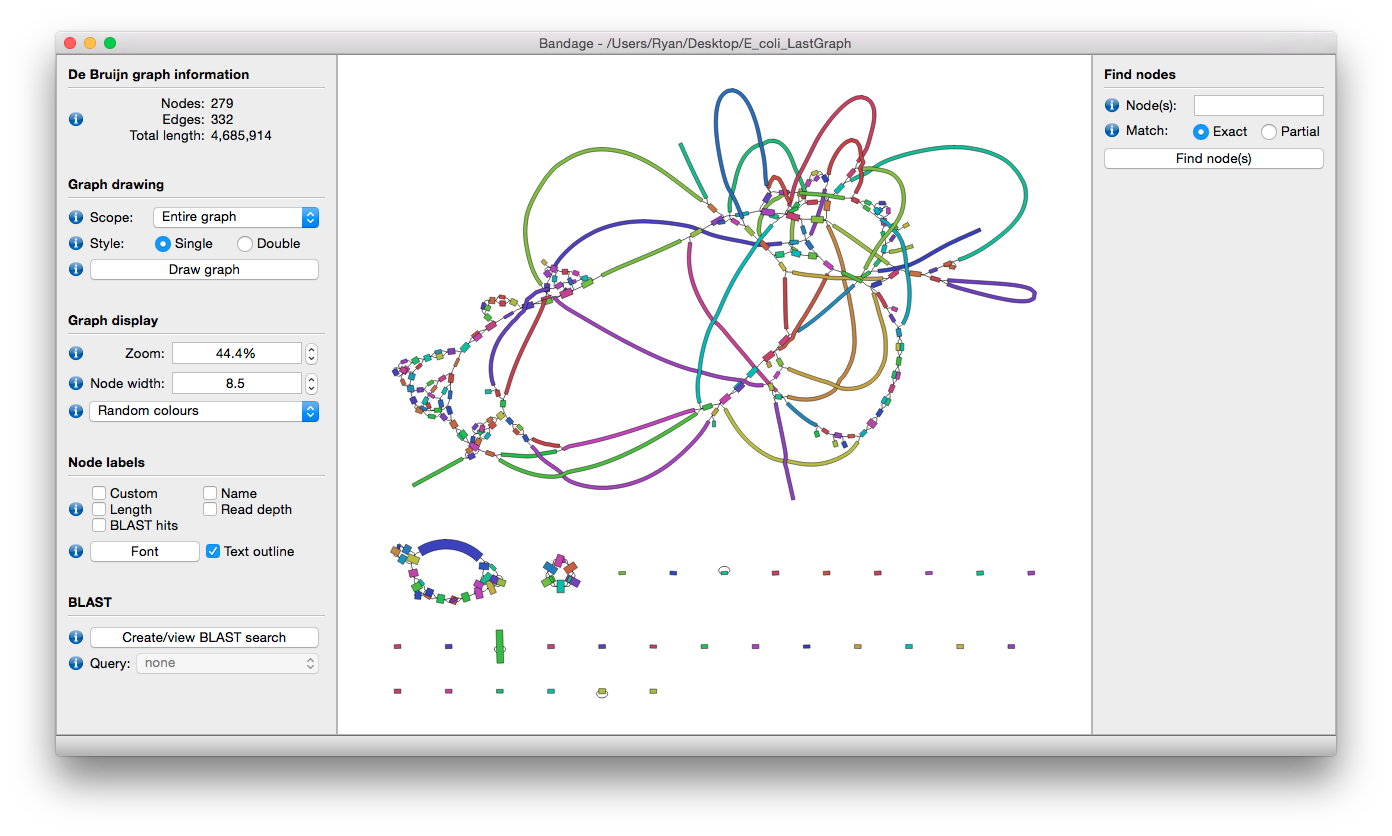
Assignment
Please upload Bandage output
PacBio assembly
conda deactivate
conda activate preprocessing
conda install -c conda-forge -c anaconda -c bioconda nanostat nanoplot
Reads download
cd /data/gpfs/assoc/bch709-1/<YOURID>/Genome_assembly/
mkdir PacBio
cd PacBio
/data/gpfs/assoc/bch709-1/Course_material/2020/PacBio/BCH709_Pacbio_01.fastq.gz
/data/gpfs/assoc/bch709-1/Course_material/2020/PacBio/BCH709_Pacbio_02.fastq.gz
Check PacBio reads statistics
NanoStat --fastq BCH709_Pacbio_01.fastq.gz BCH709_Pacbio_02.fastq.gz -t 2
NanoPlot -t 2 --fastq  bch709-1_Pacbio_01.fastq.gz bch709-1_Pacbio_02.fastq.gz  --maxlength 40000 --plots hex dot pauvre -o pacbio_stat
Transfer your result
*.png *.html *.txt
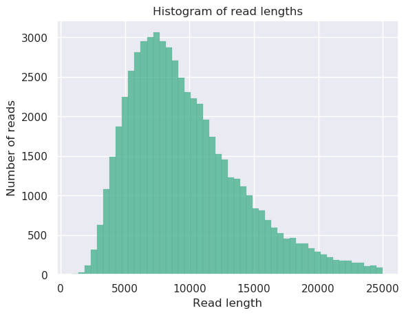
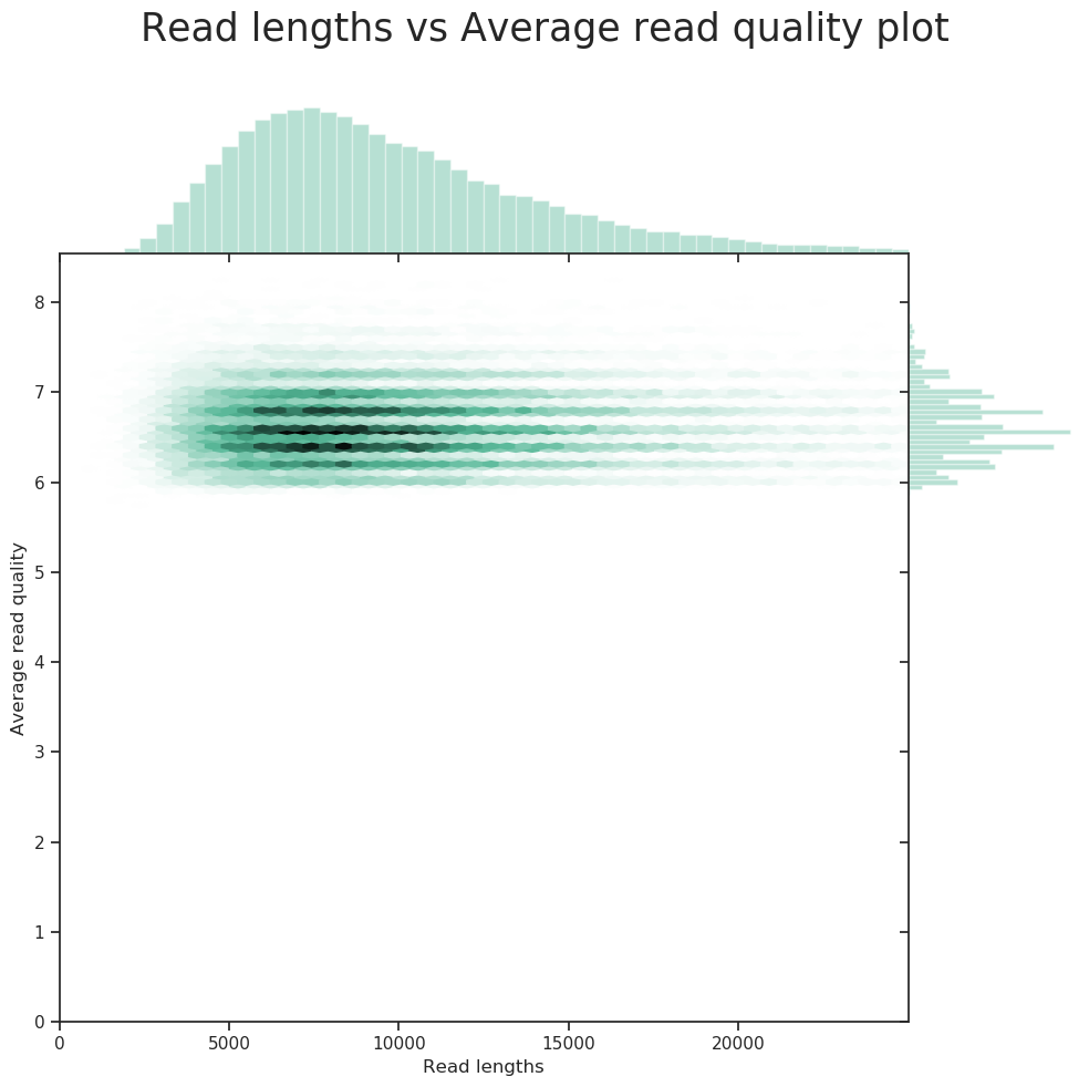
PacBio reads statistics
General summary:
Mean read length:               9,698.6
Mean read quality:                  6.6
Median read length:             8,854.0
Median read quality:                6.6
Number of reads:               58,497.0
Read length N50:               10,901.0
Total bases:              567,339,600.0
Number, percentage and megabases of reads above quality cutoffs
>Q5:	58497 (100.0%) 567.3Mb
>Q7:	8260 (14.1%) 78.6Mb
>Q10:	0 (0.0%) 0.0Mb
>Q12:	0 (0.0%) 0.0Mb
>Q15:	0 (0.0%) 0.0Mb
Top 5 highest mean basecall quality scores and their read lengths
1:	8.5 (13544)
2:	8.5 (14158)
3:	8.5 (9590)
4:	8.5 (10741)
5:	8.5 (7529)
Top 5 longest reads and their mean basecall quality score
1:	24999 (6.4)
2:	24992 (6.0)
3:	24983 (7.0)
4:	24980 (6.5)
5:	24977 (6.6)
Hybrid Genome assembly Spades
cd /data/gpfs/assoc/bch709-1/<YOURID>/Genome_assembly/

mkdir Spades_Illumina_Pacbio
cd Spades_Illumina_Pacbio
conda activate genomeassembly
Submit below job
#!/bin/bash
#SBATCH --job-name=Spades
#SBATCH --cpus-per-task=16
#SBATCH --time=12:00:00
#SBATCH --mem=64g
#SBATCH --account=cpu-s2-bch709-1
#SBATCH --partition=cpu-s2-core-0
#SBATCH --mail-type=all
#SBATCH --mail-user=<YOUR ID>@unr.edu
#SBATCH -o Spades.out # STDOUT
#SBATCH -e Spades.err # STDERR
zcat  <BCH709_Pacbio_01.fastq.gz> <BCH709_Pacbio_02.fastq.gz> >> merged_pacbio.fastq
spades.py -k 21,33,55,77 --careful -1 <trim_galore output> -2 <trim_galore output> --pacbio merged_pacbio.fastq -o spades_output --memory 64 --threads 16
De novo assembly
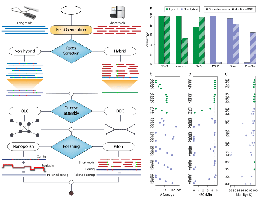
Canu
Canu (Koren et al. 2017) is a fork of the celera assembler and improves upon the earlier PBcR pipeline into a single, comprehensive assembler. Highly repetitive k-mers, which are abundant in all the reads, can be non-informative. Hence term frequency, inverse document frequency (tf-idf), a weighting statistic was added to MinHashing, giving weightage to non-repetitive k-mers as minimum values in the MinHash sketches, and sensitivity has been demonstrated to reach up to 89% without any parameter adjustment. By retrospectively inspecting the assembly graphs and also statistically filtering out repeat-induced overlaps, the chances of mis-assemblies are reduced.
Canu assembly
cd /data/gpfs/assoc/bch709-1/<YOURID>/Genome_assembly/PacBio
conda activate genomeassembly
Submit below job
#!/bin/bash
#SBATCH --job-name=Canu
#SBATCH --cpus-per-task=8
#SBATCH --time=2:00:00
#SBATCH --mem=24g
#SBATCH --account=cpu-s2-bch709-1
#SBATCH --partition=cpu-s2-core-0
#SBATCH --mail-type=all
#SBATCH --mail-user=<YOUR ID>@unr.edu
#SBATCH -o Canu.out # STDOUT
#SBATCH -e Canu.err # STDERR

canu -p canu -d canu_outdir genomeSize=11m -pacbio <LOCATION_BCH709_Pacbio_1.fastq.gz> <LOCATION_BCH709_Pacbio_1.fastq.gz> corThreads=8 batMemory=64  ovbMemory=32 ovbThreads=8 corOutCoverage=32  ovsMemory=32-186 maxMemory=128 ovsThreads=8 oeaMemory=16  executiveMemory=32 gridOptions='--time=12-00:00:00 -p cpu-s2-core-0 -A cpu-s2-bch709-1 --mail-type=all --mail-user=<YOUR ID>@unr.edu'
Check the Quality of Genome Assembly
cd /data/gpfs/assoc/bch709-1/<YOURID>/Genome_assembly/
mkdir genomeassembly_results/
cd genomeassembly_results
Activate Your environment
conda activate genomeassembly
Copy Your Assembly Results
Spades
cp /data/gpfs/assoc/bch709-1/<YOURID>/Genome_assembly/Spades_Illumina_Pacbio/spades_output/scaffolds.fasta spades_pacbio_illumina.fasta

cp /data/gpfs/assoc/bch709-1/<YOURID>/Genome_assembly/Illumina/Spades/spades_output/scaffolds.fasta spades_illumina.fasta
Canu
cp /data/gpfs/assoc/bch709-1/<YOURID>/Genome_assembly/PacBio/canu_outdir/canu.contigs.fasta canu.contigs.fasta
Canu results
cp /data/gpfs/assoc/bch709-1/Course_material/2020/Genome_assembly/canu.contigs.fasta canu.contigs.fasta
Check Your Assembly Results
assembly-stats canu.contigs.fasta spades_pacbio_illumina.fasta spades_illumina.fasta
Compare Assemblies
Install Global Alignmnet Software
cd /data/gpfs/assoc/bch709-1/<YOURID>/Genome_assembly/
mkdir genomeassembly_alignment/
cd genomeassembly_alignment
conda activate genomeassembly
conda install  -c conda-forge -c anaconda -c bioconda mummer -y
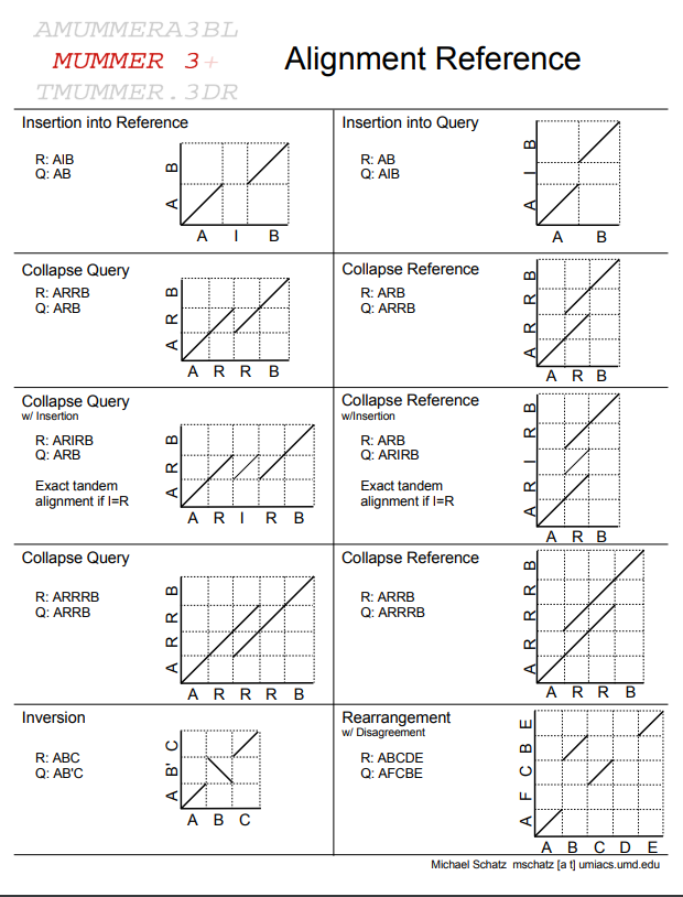
Open source MUMmer 3.0 is described in “Versatile and open software for comparing large genomes.” S. Kurtz, A. Phillippy, A.L. Delcher, M. Smoot, M. Shumway, C. Antonescu, and S.L. Salzberg, Genome Biology (2004), 5:R12.
MUMmer 2.1, NUCmer, and PROmer are described in “Fast Algorithms for Large-scale Genome Alignment and Comparision.” A.L. Delcher, A. Phillippy, J. Carlton, and S.L. Salzberg, Nucleic Acids Research (2002), Vol. 30, No. 11 2478-2483.
MUMmer 1.0 is described in “Alignment of Whole Genomes.” A.L. Delcher, S. Kasif, R.D. Fleischmann, J. Peterson, O. White, and S.L. Salzberg, Nucleic Acids Research, 27:11 (1999), 2369-2376.
Space efficent suffix trees are described in “Reducing the Space Requirement of Suffix Trees.” S. Kurtz, Software-Practice and Experience, 29(13): 1149-1171, 1999.
Run Genome Wide Global Alignmnet Software
#!/bin/bash
#SBATCH --job-name=nucmer
#SBATCH --cpus-per-task=2
#SBATCH --time=15:00
#SBATCH --mem=10g
#SBATCH --mail-type=all
#SBATCH --mail-user=<YOURID>@unr.edu
#SBATCH -o nucmer.out # STDOUT
#SBATCH -e nucmer.err # STDERR
#SBATCH --account=cpu-s6-test-0
#SBATCH --partition=cpu-s6-test-0
nucmer  --coords -p canu_pacbio_Spades_illumina <canu.contigs> <illumina_spades_scaffold_file>


nucmer  --coords -p canu_pacbio_Spades_illumina_pacbio <canu.contigs> <Spades_illumina_pacbio_scaffold_file>
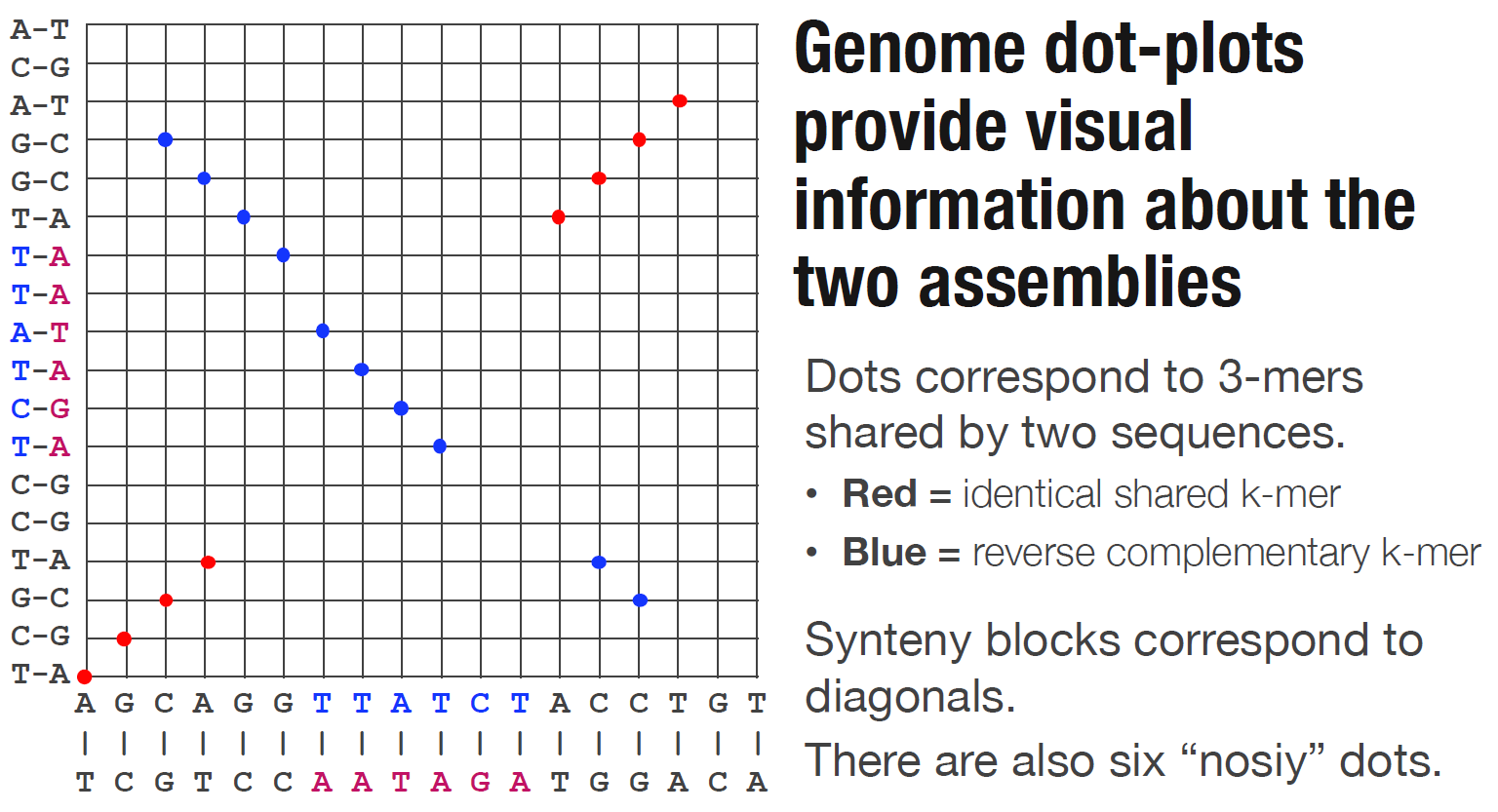
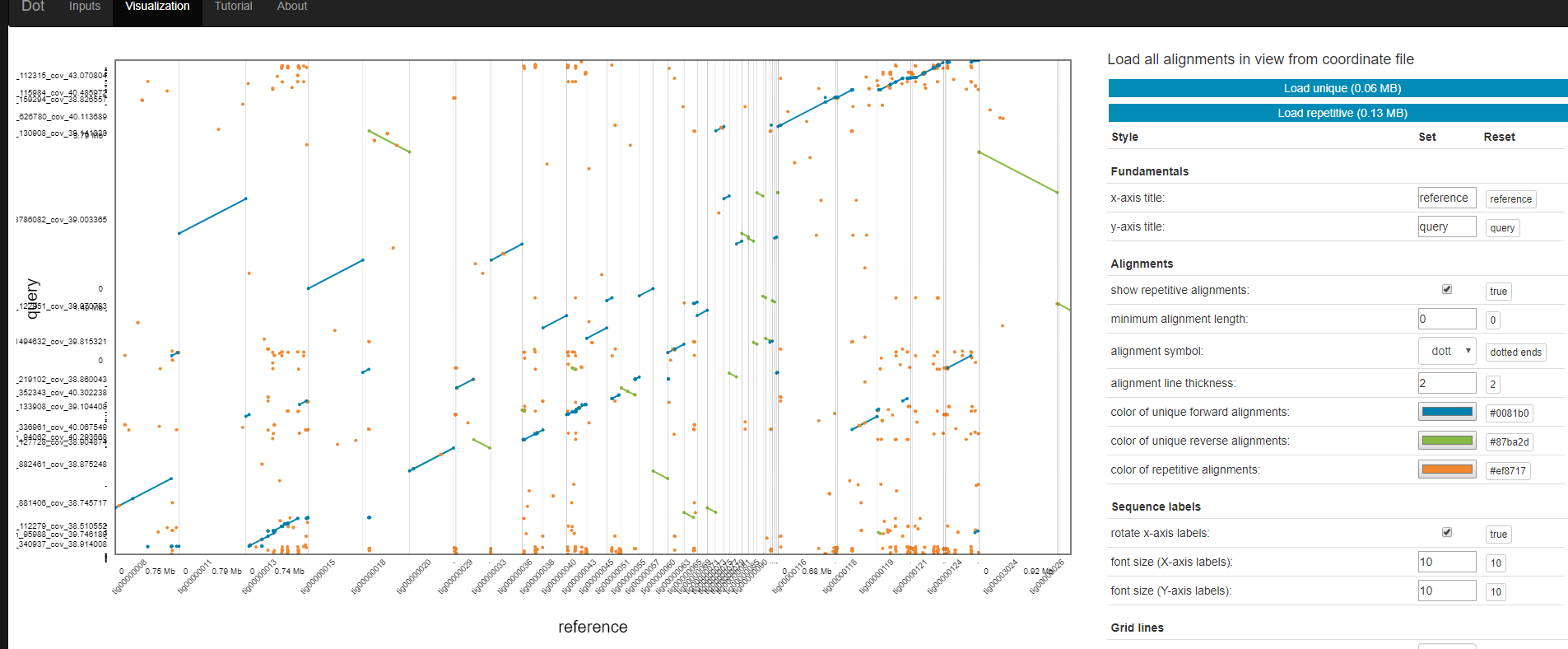
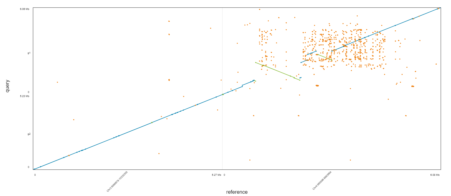
Dot
Dot is an interactive dot plot viewer for genome-genome alignments.
Dot is publicly available here: https://dnanexus.github.io/dot And can also be used locally by cloning this repository and simply opening the index.html file in a web browser.
After aligning genome assemblies or finished genomes against each other with MUMmer’s nucmer, the alignments can be visualized with Dot. Instead of generating static dot plot images on the command-line, Dot lets you interact with the alignments by zooming in and investigating regions in detail.
To prepare a .delta file (nucmer output) for Dot, run this python (3.6) script first: https://dnanexus.github.io/dot/DotPrep.py
The DotPrep.py script will apply a unique anchor filtering algorithm to mark alignments as unique or repetitive. This algorithm analyzes all of the alignments, and it needs to see unfiltered data to determine which alignments are repetitive, so make sure to run nucmer without any filtering options and without running delta-filter on the .delta file before passing it into DotPrep.py.
wget https://dnanexus.github.io/dot/DotPrep.py

chmod 775 DotPrep.py
nano DotPrep.sh
#!/bin/bash
#SBATCH --job-name=dot
#SBATCH --cpus-per-task=2
#SBATCH --time=15:00
#SBATCH --mem=10g
#SBATCH --mail-type=all
#SBATCH --mail-user=wyim@unr.edu
#SBATCH -o nucmer.out # STDOUT
#SBATCH -e nucmer.err # STDERR
#SBATCH --account=cpu-s6-test-0
#SBATCH --partition=cpu-s6-test-0
python DotPrep.py  --delta canu_pacbio_Spades_illumina.delta --out  canu_pacbio_Spades_illumina
python DotPrep.py  --delta canu_pacbio_Spades_illumina_pacbio.delta  --out canu_pacbio_Spades_illumina_pacbio
The output of DotPrep.py includes the *.coords and *.coords.idx that should be used with Dot for visualization.
Visualization
- Transfer *.coords.* files
- Go to https://dnanexus.github.io/dot/
The output of DotPrep.py includes the *.coords and *.coords.idx that should be used with Dot for visualization.
Which one is the best?
Assignment
Please upload three dot plot from assembly comparison.
-
Download below file. https://www.dropbox.com/s/xpnhj6j99dr1kum/Athaliana_subset_bch709-1.fa.
-
Align three fasta files (spades_illumina.fasta, spades_pacbio_illumina.fasta, canu.contigs.fasta) to downloaded Athaliana_subset_bch709-1.fa by nucmer independently.
-
Generate coords and coords.idx file using DotPrep.py.
-
Draw dot plot by DOT website.
-
Upload three dotplot to Webcanvas.
wget https://www.dropbox.com/s/xpnhj6j99dr1kum/Athaliana_subset_bch709-1.fa
Pilon
cd /data/gpfs/assoc/bch709-1/<YOURID>/Genome_assembly/
mkdir Pilon
cd Pilon

conda deactivate
conda create -n postprocess python=3 -y
conda activate postprocess
conda install -y -c conda-forge -c anaconda -c bioconda pilon bwa samtools openssl=1.0
## at your genome assembly folder
Pilon uses read alignment analysis to diagnose, report, and automatically improve de novo genome assemblies as well as call variants. Pilon then outputs a FASTA file containing an improved representation of the genome from the read data and an optional VCF file detailing variation seen between the read data and the input genome.
To aid manual inspection and improvement by an analyst, Pilon can optionally produce tracks that can be displayed in genome viewers such as IGV and GenomeView, and it reports other events (such as possible large collapsed repeat regions) in its standard output.
nano mapping.sh
#!/bin/bash
#SBATCH --job-name=Illumina_mapping
#SBATCH --cpus-per-task=16
#SBATCH --time=12:00:00
#SBATCH --mem=20g
#SBATCH --mail-type=all
#SBATCH --mail-user=<YOUREMAIL>
#SBATCH -o mapping.out # STDOUT
#SBATCH -e mapping.err # STDERR
#SBATCH -p cpu-s2-core-0
#SBATCH -A cpu-s2-bch709-1
#ln -s /data/gpfs/assoc/bch709-1/<YOURID>/Genome_assembly/genomeassembly_results/canu.contigs.fasta /data/gpfs/assoc/bch709-1/<YOURID>/Genome_assembly/Pilon

ln -s /data/gpfs/assoc/bch709-1/Course_material/2020/Genome_assembly/canu.contigs.fasta /data/gpfs/assoc/bch709-1/<YOURID>/Genome_assembly/Pilon

bwa index canu.contigs.fasta

bwa mem -t 24  canu.contigs.fasta  <Trimmed_illumina_R1 val something> <Trimmed_illumina_R2 val something>  -o canu_illumina.sam
samtools view -Sb canu_illumina.sam -o canu_illumina.bam
samtools sort canu_illumina.bam -o canu_illumina_sort.bam
samtools index canu_illumina_sort.bam
samtools faidx canu.contigs.fasta
nano /data/gpfs/home/<YOURID>/miniconda3/envs/postprocess/bin/pilon


default_jvm_mem_opts = ['-Xms8g', '-Xmx40g']
nano pilon.sh
#!/bin/bash
#SBATCH --job-name=pilon
#SBATCH --cpus-per-task=16
#SBATCH --time=12:00:00
#SBATCH --mem=40g
#SBATCH --mail-type=all
#SBATCH --mail-user=<YOUREMAIL>
#SBATCH -o pilon.out # STDOUT
#SBATCH -e pilon.err # STDERR
#SBATCH -p cpu-s2-core-0
#SBATCH -A cpu-s2-bch709-1

pilon --genome canu.contigs.fasta --frags canu_illumina_sort.bam --output canu.illumina  --vcf --changes --threads 16
sbatch --dependency=afterok:<123456> pilon.sh
nano mapping_new.sh
#!/bin/bash
#SBATCH --job-name=Illumina_mapping
#SBATCH --cpus-per-task=16
#SBATCH --time=12:00:00
#SBATCH --mem=20g
#SBATCH --mail-type=all
#SBATCH --mail-user=<YOUREMAIL>
#SBATCH -o mapping.out # STDOUT
#SBATCH -e mapping.err # STDERR
#SBATCH -p cpu-s2-core-0
#SBATCH -A cpu-s2-bch709-1

bwa index canu.illumina.fasta

bwa mem -t 24 canu.illumina.fasta  <Trimmed_illumina_R1 val something> <Trimmed_illumina_R2 val something>  -o canu_illumina_pilon.sam
samtools view -Sb canu_illumina_pilon.sam -o canu_illumina_pilon.bam
samtools sort canu_illumina_pilon.bam -o canu_illumina_pilon_sort.bam
samtools index canu_illumina_pilon_sort.bam
samtools faidx canu.illumina.fasta
############
Visualization
http://software.broadinstitute.org/software/igv/
The Integrative Genomics Viewer (IGV) is a high-performance visualization tool for interactive exploration of large, integrated genomic datasets. It supports a wide variety of data types, including array-based and next-generation sequence data, and genomic annotations.
IGV is available in multiple forms, including:
the original IGV - a Java desktop application, IGV-Web - a web application, igv.js - a JavaScript component that can be embedded in web pages (for developers)
http://software.broadinstitute.org/software/igv/download
cd /data/gpfs/assoc/bch709-1/<YOUID>/Genome_assembly/Pilon

mkdir PrePilon
mkdir PostPilon

cp canu_illumina_pilon_sort.bam canu_illumina_pilon_sort.bam.bai canu.illumina.fasta canu.illumina.fasta.fai PostPilon

cp canu_illumina_sort.bam canu_illumina_sort.bam.bai canu.contigs.fasta canu.contigs.fasta.fai PrePilon
Local computer Download For Visualization
canu_illumina_pilon_sort.bam canu_illumina_pilon_sort.bam.bai canu.illumina.fasta canu.illumina.fasta.fai

canu_illumina_sort.bam canu_illumina_sort.bam.bai canu.contigs.fasta canu.contigs.fasta.fai
conda activate postprocess
conda install -c bioconda -c conda-forge htslib=1.9
bgzip -@ 2 canu.illumina.vcf
tabix -p vcf canu.illumina.vcf.gz
Investigate taxa
Here we introduce a software called Kraken2. This tool uses k-mers to assign a taxonomic labels in form of NCBI Taxonomy to the sequence (if possible). The taxonomic label is assigned based on similar k-mer content of the sequence in question to the k-mer content of reference genome sequence. The result is a classification of the sequence in question to the most likely taxonomic label. If the k-mer content is not similar to any genomic sequence in the database used, it will not assign any taxonomic label.
cd /data/gpfs/assoc/bch709-1/<YOURID>/Genome_assembly/
mkdir taxa
cd taxa

conda deactivate
conda create -n taxa -y python=3.6
conda activate taxa
conda install -c r -c conda-forge -c anaconda -c bioconda kraken kraken2 -y
We can also use another tool by the same group called Centrifuge. This tool uses a novel indexing scheme based on the Burrows-Wheeler transform (BWT) and the Ferragina-Manzini (FM) index, optimized specifically for the metagenomic classification problem to assign a taxonomic labels in form of NCBI Taxonomy to the sequence (if possible). The result is a classification of the sequence in question to the most likely taxonomic label. If the search sequence is not similar to any genomic sequence in the database used, it will not assign any taxonomic label.
conda install -c bioconda centrifuge -y
#!/bin/bash
#SBATCH --job-name=centrifuge
#SBATCH --cpus-per-task=24
#SBATCH --time=12:00:00
#SBATCH --mem=220g
#SBATCH --mail-type=all
#SBATCH --mail-user=wyim@unr.edu
#SBATCH -o centrifuge.out # STDOUT
#SBATCH -e centrifuge.err # STDERR
#SBATCH -p cpu-s2-core-0
#SBATCH -A cpu-s2-bch709-1
centrifuge -x /data/gpfs/assoc/bch709-1/Course_material/2020/taxa/nt  -1 /data/gpfs/assoc/bch709-1/<YOURID>/Genome_assembly/Illumina/trimmed_fastq/WGS_R1_val_1.fq  -2 /data/gpfs/assoc/bch709-1/<YOURID>/Genome_assembly/Illumina/trimmed_fastq/WGS_R2_val_2.fq  --report-file taxa.illumina --threads 24
#!/bin/bash
#SBATCH --job-name=centrifuge
#SBATCH --cpus-per-task=1
#SBATCH --time=12:00:00
#SBATCH --mem=10g
#SBATCH --mail-type=all
#SBATCH --mail-user=wyim@unr.edu
#SBATCH -o centrifuge.out # STDOUT
#SBATCH -e centrifuge.err # STDERR
#SBATCH -p cpu-s2-core-0
#SBATCH -A cpu-s2-bch709-1
centrifuge-kreport  -x  /data/gpfs/assoc/bch709-1/Course_material/2020/taxa/nt  taxa.illumina > taxa.illumina_kraken
Centrifuge report
https://fbreitwieser.shinyapps.io/pavian/
BUSCO
BUSCO assessments are implemented in open-source software, with a large selection of lineage-specific sets of Benchmarking Universal Single-Copy Orthologs. These conserved orthologs are ideal candidates for large-scale phylogenomics studies, and the annotated BUSCO gene models built during genome assessments provide a comprehensive gene predictor training set for use as part of genome annotation pipelines.
https://busco.ezlab.org/
cd /data/gpfs/assoc/bch709-1/<YOURID>/Genome_assembly/
mkdir BUSCO
cd BUSCO
cp /data/gpfs/assoc/bch709-1/<YOURID>/Genome_assembly/genomeassembly_results/*.fasta .
 cp /data/gpfs/assoc/bch709-1/<YOURID>/Genome_assembly/Pilon/canu.illumina.fasta .

conda create -n busco4  python=3.6
conda activate busco4
conda install -c bioconda -c conda-forge busco=4.0.5 'multiqc<1.34' biopython
#!/bin/bash
#SBATCH --job-name=busco
#SBATCH --cpus-per-task=24
#SBATCH --time=12:00:00
#SBATCH --mem=20g
#SBATCH --mail-type=all
#SBATCH --mail-user=wyim@unr.edu
#SBATCH -o busco.out # STDOUT
#SBATCH -e busco.err # STDERR
#SBATCH -p cpu-s2-core-0
#SBATCH -A cpu-s2-bch709-1

export AUGUSTUS_CONFIG_PATH="~/miniconda3/envs/busco4/config/"

busco -l viridiplantae_odb10 --cpu 24 --in spades_illumina.fasta --out BUSCO_Illumina --mode genome  -f

busco -l viridiplantae_odb10 --cpu 24 --in spades_pacbio_illumina.fasta --out BUSCO_Illumina_Pacbio --mode genome  -f

busco -l viridiplantae_odb10 --cpu 24 --in canu.contigs.fasta   --out BUSCO_Pacbio --mode genome  -f

busco -l viridiplantae_odb10 --cpu 24 --in canu.illumina.fasta   --out BUSCO_Pacbio_Pilon --mode genome  -f

multiqc . -n assembly --exclude rsem --exclude gatk
BUSCO results
INFO:   Results:        C:10.8%[S:10.8%,D:0.0%],F:0.5%,M:88.7%,n:425

INFO:

        --------------------------------------------------
        |Results from dataset viridiplantae_odb10         |
        --------------------------------------------------
        |C:10.8%[S:10.8%,D:0.0%],F:0.5%,M:88.7%,n:425     |
        |46     Complete BUSCOs (C)                       |
        |46     Complete and single-copy BUSCOs (S)       |
        |0      Complete and duplicated BUSCOs (D)        |
        |2      Fragmented BUSCOs (F)                     |
        |377    Missing BUSCOs (M)                        |
        |425    Total BUSCO groups searched               |
        --------------------------------------------------
INFO:   BUSCO analysis done. Total running time: 123 seconds
mkdir BUSCO_result
cp BUSCO_*/*.txt BUSCO_result
generate_plot.py -wd BUSCO_result
Chromosome assembly
cd  /data/gpfs/assoc/bch709-1/<YOURID>/Genome_assembly/
mkdir /data/gpfs/assoc/bch709-1/<YOURID>/Genome_assembly/hic   ## will go to genome assembly folder adn make hic folder
cd !$
How can we improve these genome assemblies?
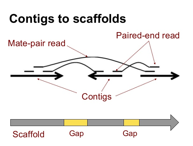
Mate Pair Sequencing
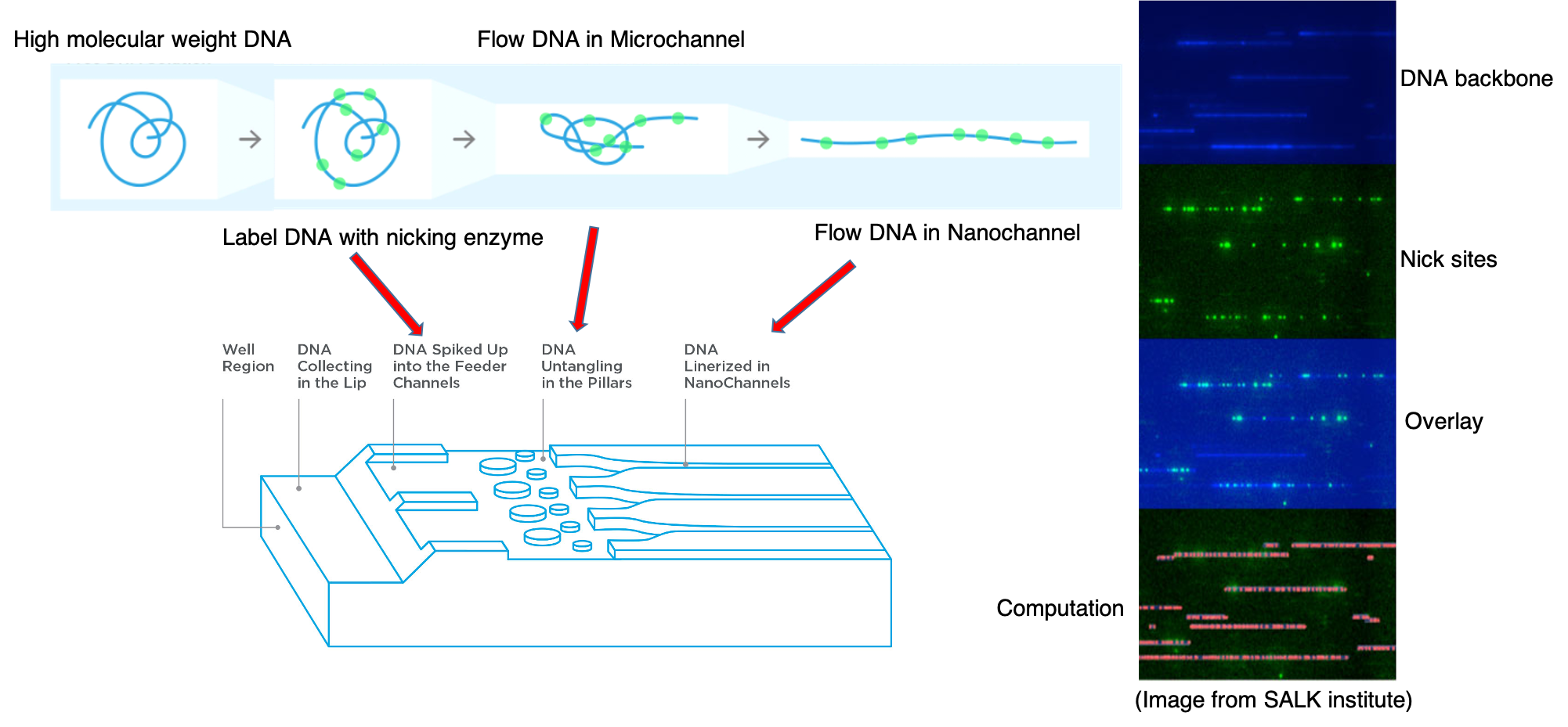
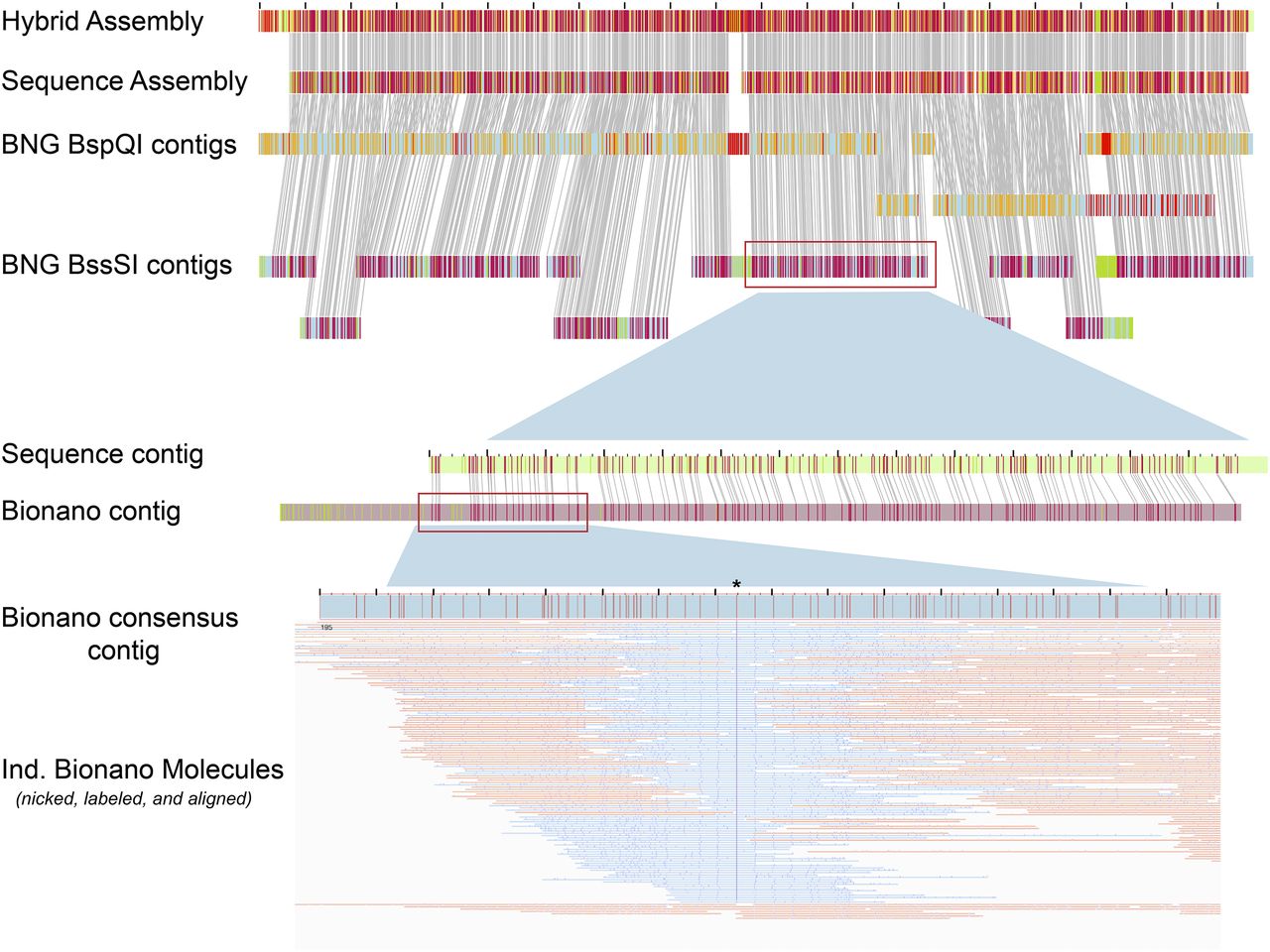
BioNano Optical Mapping
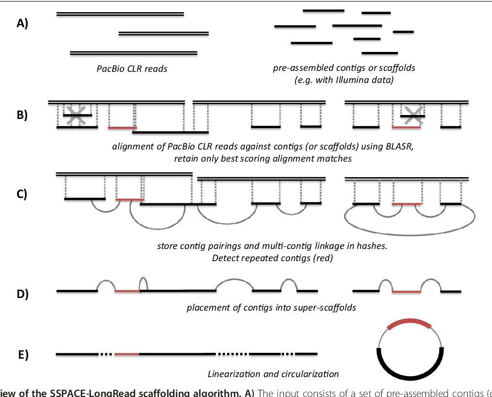
Long Read Scaffolding
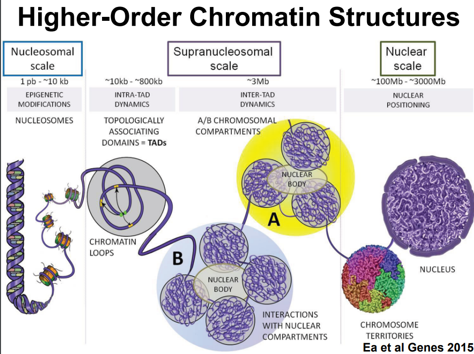
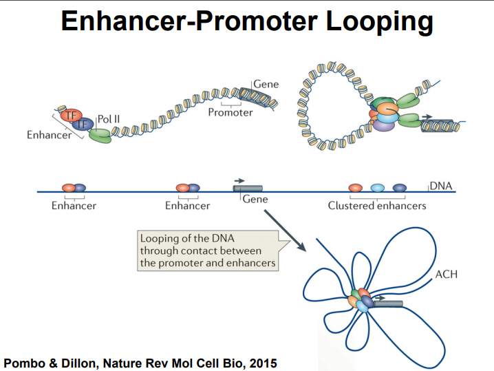
Chromosome Conformation Scaffolding
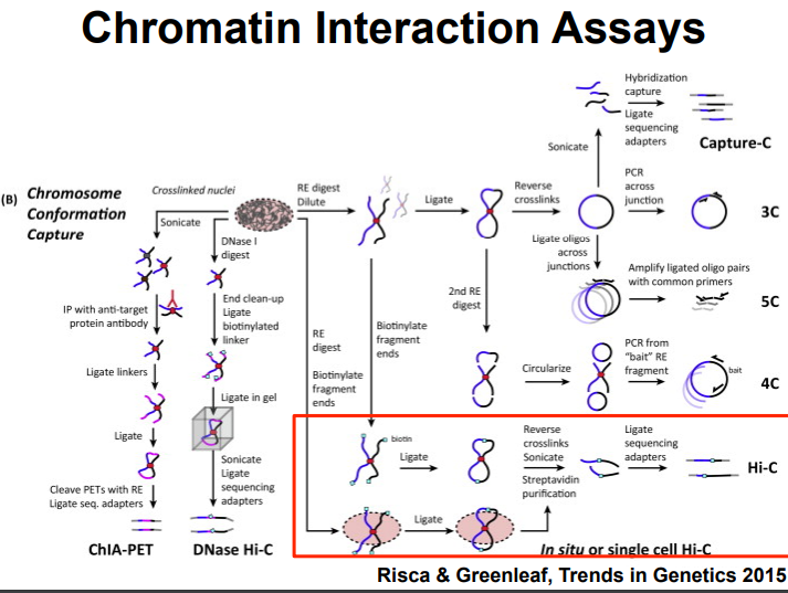
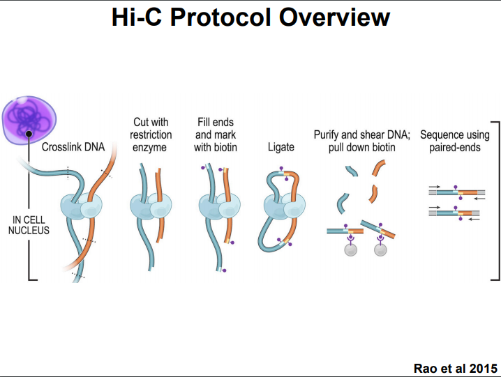
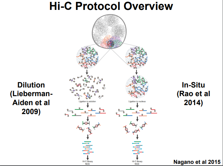
HiC for Genome Assembly
Chromosome assembly
mkdir /data/gpfs/assoc/bch709-1/<YOURID>/Genome_assembly/Hic
cd !$
HiC
conda create -n hic

conda activate hic

conda install -c r -c conda-forge -c anaconda -c bioconda samtools bedtools matplotlib numpy scipy bwa openssl=1.0 -y
canu.illumina.fasta
The input of HiC is the output of Pilon. If you don’t have it please do Pilon first.
File preparation
cp /data/gpfs/assoc/bch709-1/Course_material/2020/Genome_assembly/hic_r{1,2}.fastq.gz .

cp /data/gpfs/assoc/bch709-1/Course_material/2020/Genome_assembly/allhic.zip .
ALLHiC
Phasing and scaffolding polyploid genomes based on Hi-C data
Introduction
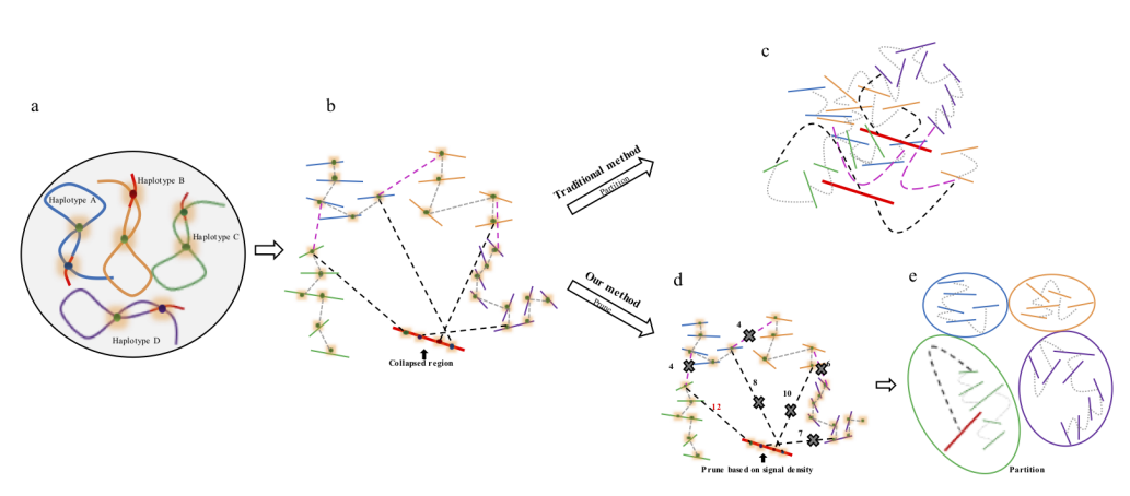
The major problem of scaffolding polyploid genome is that Hi-C signals are frequently detected between allelic haplotypes and any existing stat of art Hi-C scaffolding program links the allelic haplotypes together. To solve the problem, we developed a new Hi-C scaffolding pipeline, called ALLHIC, specifically tailored to the polyploid genomes. ALLHIC pipeline contains a total of 5 steps: prune, partition, rescue, optimize and build.
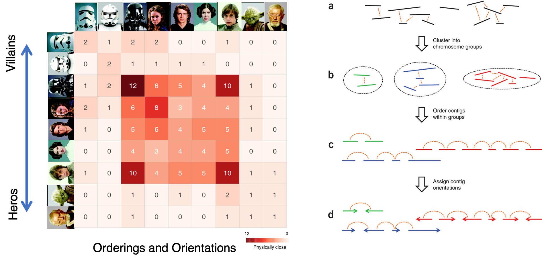
Overview of ALLHiC

Figure 1. Overview of major steps in ALLHiC algorithm. The newly released ALLHiC pipeline contains a total of 5 functions: prune, partition, rescue, optimize and build. Briefly, the prune step removes the inter-allelic links so that the homologous chromosomes are more easily separated individually. The partition function takes pruned bam file as input and clusters the linked contigs based on the linkage suggested by Hi-C, presumably along the same homologous chromosome in a preset number of partitions. The rescue function searches for contigs that are not involved in partition step from original un-pruned bam files and assigned them to specific clusters according Hi-C signal density. The optimize step takes each partition, and optimize the ordering and orientations for all the contigs. Finally, the build step reconstructs each chromosome by concatenating the contigs, adding gaps between the contigs and generating the final genome release in FASTA format.
Explanation of Prune
Prune function will firstly allow us to detect allelic contigs, which can be achieved by identifying syntenic genes based on a well-assembled close related species or an assembled monoploid genome. Signals (normalized Hi-C reads) between allelic contigs are removed from the input BAM files. In polyploid genome assembly, haplotypes that share high similarity are likely to be collapsed. Signals between the collapsed regions and nearby phased haplotypes result in chimeric scaffolds. In the prune step, only the best linkage between collapsed coting and phased contig is retained.
 Figure 2. Description of Hi-C scaffolding problem in polyploid genome and application of prune approach for haplotype phasing. (a) a schematic diagram of auto-tetraploid genome. Four homologous chromosomes are indicated as different colors (blue, orange, green and purple, respectively). Red regions in the chromosomes indicate sequences with high similarity. (b) Detection of Hi-C signals in the auto-tetraploid genome. Black dash lines indicate Hi-C signals between collapsed regions and un-collpased contigs. Pink dash lines indicate inter-haplotype Hi-C links and grey dash lines indicate intra-haplotype Hi-C links. During assembly, red regions will be collapsed due to high sequence similarity; while, other regions will be separated into different contigs if they have abundant variations. Since the collapsed regions are physically related with contigs from different haplotypes, Hi-C signals will be detected between collapsed regions with all other un-collapsed contigs. (c) Traditional Hi-C scaffolding methods will detect signals among contigs from different haplotypes as well as collapsed regions and cluster all the sequences together. (d) Prune Hi-C signals: 1- remove signals between allelic regions; 2- only retain the strongest signals between collapsed regions and un-collapsed contigs. (e) Partition based on pruned Hi-C information. Contigs are ideally phased into different groups based on prune results.
Citations
Zhang, X. Zhang, S. Zhao, Q. Ming, R. Tang, H. Assembly of allele-aware, chromosomal scale autopolyploid genomes based on Hi-C data. Nature Plants, doi:10.1038/s41477-019-0487-8 (2019).
Zhang, J. Zhang, X. Tang, H. Zhang, Q. et al. Allele-defined genome of the autopolyploid sugarcane Saccharum spontaneum L. Nature Genetics, doi:10.1038/s41588-018-0237-2 (2018).
Algorithm demo
Solving scaffold ordering and orientation (OO) in general is NP-hard. ALLMAPS converts the problem into Traveling Salesman Problem (TSP) and refines scaffold OO using Genetic Algorithm. For rough idea, a ‘live’ demo of the scaffold OO on yellow catfish chromosome 1 can be viewed in the animation below.

Traveling Salesman Problem
Run AllHIC -> hic.sh
#!/bin/bash
#SBATCH --job-name=AllHIC
#SBATCH --cpus-per-task=24
#SBATCH --time=12:00:00
#SBATCH --mem=48g
#SBATCH --mail-type=all
#SBATCH --mail-user=<YOUREMAIL>
#SBATCH -o hic.out # STDOUT
#SBATCH -e hic.err # STDERR
#SBATCH -p cpu-s2-core-0
#SBATCH -A cpu-s2-bch709-1
unzip allhic.zip
chmod 775 ALL* all*

cp /data/gpfs/assoc/bch709-1/<YOURID>/Genome_assembly/Pilon/canu.illumina.fasta .

bwa index canu.illumina.fasta
bwa mem -t 24 -SPM canu.illumina.fasta hic_r1.fastq.gz hic_r2.fastq.gz  > hic.sam
samtools view -Sb hic.sam -o hic.bam -@ 24
samtools
./allhic extract hic.bam canu.illumina.fasta
./allhic partition hic.counts_GATC.txt hic.pairs.txt 2
./allhic optimize hic.counts_GATC.2g1.txt  hic.clm
./allhic optimize hic.counts_GATC.2g2.txt  hic.clm

ALLHiC_build canu.illumina.fasta

cp groups.asm.fasta bch709-1_assembly.fasta
](/fig/hicmovie.gif)